Mastering Paley's Osteotomy: Frontal Plane Realignment & Deformity Correction
Key Takeaway
Paley's osteotomy principles transform orthopedic deformity correction into a precise science. This masterclass covers frontal plane realignment, foundational biomechanics, radiographic planning, CORA, ACA, and Paley's Three Osteotomy Rules to achieve reproducible, perfect limb alignment in complex deformities.
Introduction to Frontal Plane Realignment and Paley Principles
For decades, orthopedic deformity correction was largely an intuitive art, often resulting in secondary translational deformities, joint malorientation, and residual Mechanical Axis Deviation (MAD). Surgeons would "eyeball" corrections, leading to unpredictable outcomes, altered joint biomechanics, and early onset osteoarthritis. The introduction of Dr. Dror Paley’s principles of deformity correction revolutionized the field of orthopedic surgery, transforming it into a precise, mathematically driven science.
This comprehensive masterclass delves deeply into Paley osteotomy concepts and frontal plane realignment. Whether you are managing a post-traumatic growth arrest, a congenital bowing, a complex malunion, or degenerative joint disease requiring realignment, mastering the geometric relationship between the Center of Rotation of Angulation (CORA), the Axis of Correction of Angulation (ACA), and the osteotomy level is non-negotiable for the modern orthopedic surgeon.
In this exhaustive guide, we will analyze the foundational biomechanics of the lower extremity, detail the standardized radiographic parameters required for surgical planning, and exhaustively review opening wedge, closing wedge, and dome osteotomy sequences. By rigorously applying Paley's Three Osteotomy Rules to complex distal femoral and diaphyseal deformities, surgeons can achieve reproducible, perfect alignment in every case.
Foundational Biomechanics in Orthopedic Deformity Correction
Before executing a surgical cut, the surgeon must meticulously map the mechanical and anatomic axes of the limb. Deformity planning in the frontal plane relies on a standardized set of radiographic angles, reference points, and a deep understanding of lower extremity biomechanics. The goal of any realignment surgery is to restore normal load-bearing physiology to the hip, knee, and ankle joints.
Mechanical Axis and Mechanical Axis Deviation
The mechanical axis of the lower limb is a straight line drawn from the center of the femoral head to the center of the ankle joint (the center of the tibial plafond). In a normal, well-aligned lower extremity, this line passes precisely through or slightly medial to the center of the knee joint.
Understanding the mechanical axis is the first step in the Malalignment Test.
- Mechanical Axis Deviation (MAD) If the mechanical axis passes medial or lateral to the center of the knee, the limb has Mechanical Axis Deviation.
- Medial MAD Indicates a varus deformity. The mechanical load is disproportionately shifted to the medial compartment of the knee, predisposing the patient to medial compartment arthrosis.
- Lateral MAD Indicates a valgus deformity. The mechanical load is shifted to the lateral compartment, stressing the medial collateral ligament and lateral meniscus.
Quantifying MAD is done by measuring the perpendicular distance in millimeters from the center of the knee joint to the mechanical axis line. Normal MAD is typically 1 to 8 millimeters medial to the center of the knee.
Anatomic Axis and Limb Alignment
While the mechanical axis defines the load-bearing line of the entire limb, the anatomic axis refers to the mid-diaphyseal line of an individual bone.
* In the tibia, the anatomic axis and the mechanical axis are essentially parallel and often superimposed.
* In the femur, the anatomic axis diverges from the mechanical axis by approximately 6 to 7 degrees (the anatomic-mechanical angle, or AMA).
Surgeons utilizing intramedullary nails for deformity correction must be intimately familiar with the anatomic axis, as the implant will dictate the final anatomic alignment of the bone segments.
Standardized Radiographic Joint Orientation Angles
To determine exactly where the deformity lies (femur versus tibia, proximal versus distal), the surgeon must perform the Malorientation Test. This involves measuring specific joint orientation angles and comparing them to established normal population values.
Femoral Joint Orientation Angles
The femur is evaluated by drawing the mechanical axis of the femur (from the center of the femoral head to the center of the knee) and measuring its intersection with the joint lines.
- mLDFA (mechanical Lateral Distal Femoral Angle) This is the lateral angle formed between the mechanical axis of the femur and the distal femoral joint line. The normal value is 87 degrees, with a standard range of 85 to 90 degrees. An mLDFA greater than 90 degrees indicates a distal femoral varus deformity. An mLDFA less than 85 degrees indicates a distal femoral valgus deformity.
- LPFA (Lateral Proximal Femoral Angle) This is the lateral angle formed between the mechanical axis of the femur and a line drawn from the tip of the greater trochanter to the center of the femoral head. The normal value is 90 degrees (range 85 to 95 degrees).
Tibial Joint Orientation Angles
The tibia is evaluated by drawing the mechanical axis of the tibia (from the center of the knee to the center of the ankle) and measuring its intersection with the proximal and distal joint lines.
- MPTA (Mechanical Proximal Tibial Angle) This is the medial angle formed between the mechanical axis of the tibia and the proximal tibial joint line. The normal value is 87 degrees (range 85 to 90 degrees). An MPTA less than 85 degrees indicates proximal tibial varus. An MPTA greater than 90 degrees indicates proximal tibial valgus.
- mLDTA (mechanical Lateral Distal Tibial Angle) This is the lateral angle formed between the mechanical axis of the tibia and the distal tibial joint line (tibial plafond). The normal value is 89 degrees (range 86 to 92 degrees).
Joint Line Congruency Angle
The Joint Line Congruency Angle (JLCA) is measured between the distal femoral joint line and the proximal tibial joint line. In a normal knee, these lines are nearly parallel, yielding a JLCA of 0 to 2 degrees.
A widened JLCA indicates intra-articular deformity, which may be caused by ligamentous laxity (e.g., lateral collateral ligament stretch in chronic varus) or asymmetric cartilage wear. Failing to account for a dynamic JLCA during preoperative planning will result in under-correction or over-correction of the mechanical axis.
| Radiographic Parameter | Normal Value | Pathologic Implication (High) | Pathologic Implication (Low) |
|---|---|---|---|
| mLDFA | 87° (85°-90°) | Distal Femoral Varus | Distal Femoral Valgus |
| MPTA | 87° (85°-90°) | Proximal Tibial Valgus | Proximal Tibial Varus |
| LPFA | 90° (85°-95°) | Coxa Valga | Coxa Vara |
| mLDTA | 89° (86°-92°) | Distal Tibial Valgus | Distal Tibial Varus |
| JLCA | 0°-2° | Intra-articular Deformity / Ligament Laxity | N/A |
Defining CORA and ACA in Deformity Planning
The geometric foundation of Paley's principles rests on two distinct points of reference. One is an anatomic reality of the deformed bone, and the other is a surgical choice made by the operating surgeon.
Center of Rotation of Angulation
The Center of Rotation of Angulation (CORA) represents the apex of the deformity. To find the CORA, the surgeon draws the Proximal Mechanical Axis (PMA) line and the Distal Mechanical Axis (DMA) line.
* The PMA is drawn by taking the normal joint orientation angle from the proximal joint and extending a line down the shaft.
* The DMA is drawn by taking the normal joint orientation angle from the distal joint and extending a line up the shaft.
* The exact point where the PMA and DMA intersect is the CORA.
A bone may have a single CORA (unapical deformity) or multiple CORAs (multi-apical deformity). Identifying the precise location of the CORA is the prerequisite for determining where to cut the bone and how to hinge the correction.
Axis of Correction of Angulation
While the CORA is a fixed geometric point dictated by the patient's pathology, the Axis of Correction of Angulation (ACA) is the actual hinge point around which the bone segments are rotated during surgery.
The placement of the ACA is entirely under the surgeon's control. It can be placed on the convex cortex, the concave cortex, or even outside the bone entirely (as seen with external fixator hinges). The spatial relationship between the ACA and the CORA dictates the final alignment of the limb, the presence of translation, and changes in limb length.
Paley Three Rules of Osteotomy
The cornerstone of frontal plane realignment lies in Paley's three osteotomy rules. Understanding these rules allows the surgeon to predict exactly how the mechanical axis, anatomic axis, and bone ends will shift upon correction. Mastery of these rules is what separates a master deformity surgeon from a novice.
Osteotomy Rule One Pure Angulation
The Geometric Definition
When the osteotomy line and the ACA both pass directly through the CORA, pure angular correction is achieved.
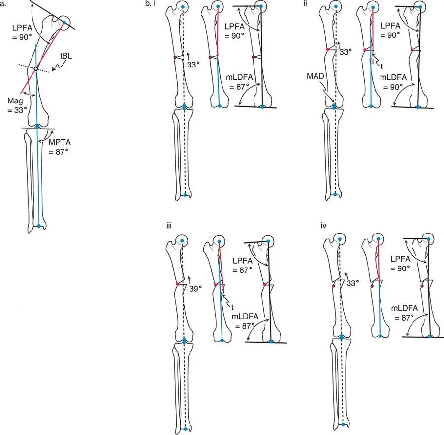
The Biomechanical Result
The mechanical axis is fully restored to normal. Because the bone is cut exactly at the apex of the deformity and hinged at that exact same apex, there is no translation of the bone segments. The anatomic axis realigns perfectly without any "step-off" or cortical bump. The proximal and distal bone segments will have maximum bony contact, promoting rapid union.
Clinical Application
This is the ideal surgical scenario. It is most easily achieved in diaphyseal deformities where the CORA lies in the midshaft, allowing the surgeon to safely cut exactly at the apex of the deformity. It is highly amenable to intramedullary nailing, as the re-established collinear anatomic axis allows for smooth passage of the guidewire and nail.
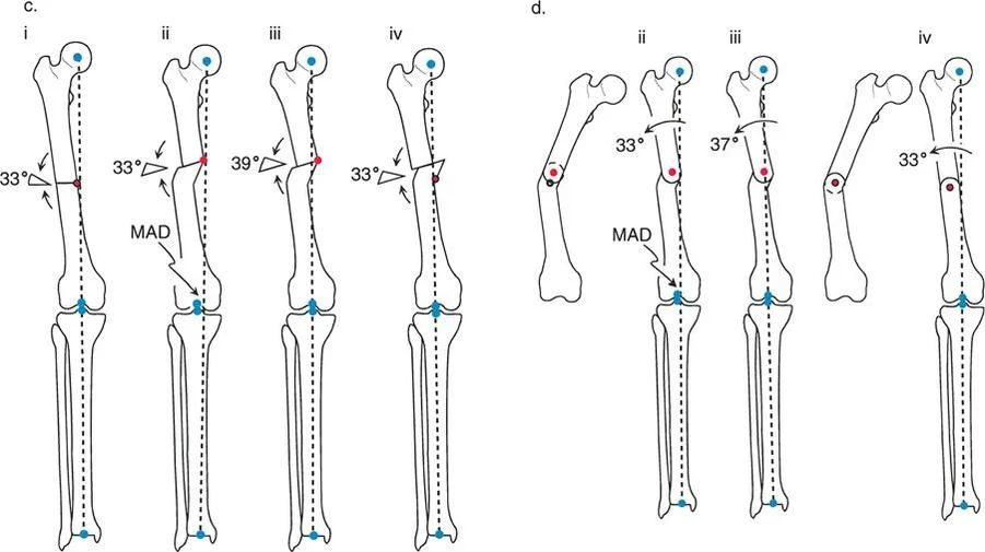
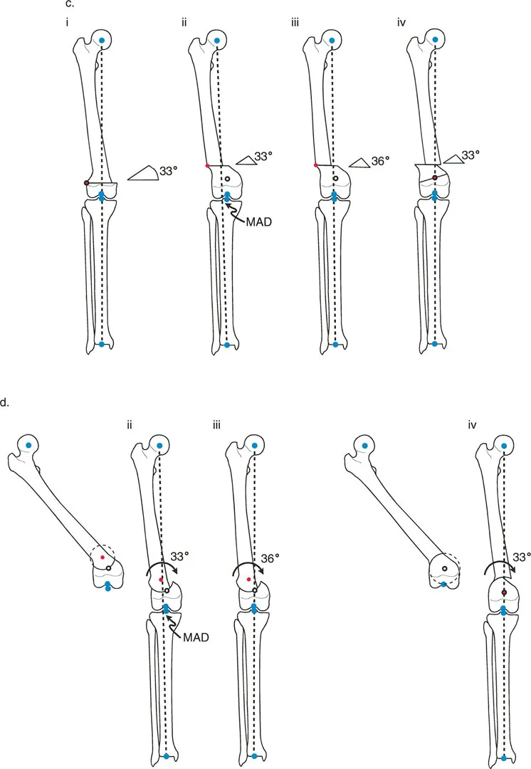
Osteotomy Rule Two Angulation with Translation
The Geometric Definition
When the ACA passes through the CORA, but the osteotomy line is made at a different level (either proximal or distal to the CORA).
The Biomechanical Result
The mechanical axis and joint orientation angles are perfectly restored. However, because the bone cut is made at a distance from the hinge point, the bone segments will mathematically translate relative to one another. This creates a visible "bump" or step-off in the anatomic axis. While the bone looks jagged on an x-ray, the load-bearing mechanical axis is flawless.
Clinical Application
Rule Two is frequently used for juxta-articular deformities. For example, if a patient has a severe distal femoral valgus deformity, the CORA may be located inside the knee joint. A surgeon cannot perform an osteotomy through the articular cartilage. Therefore, the surgeon must place the ACA at the joint (the true CORA) but perform the actual bone cut (osteotomy) safely in the metaphysis.
The resulting translation is not an error; it is a necessary and mathematically sound compromise to achieve a straight mechanical axis while cutting the bone in a biologically safe zone.
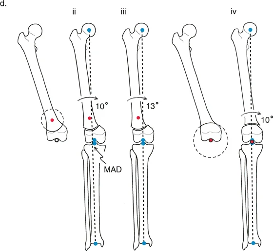
Osteotomy Rule Three Secondary Deformity
The Geometric Definition
When the osteotomy line and the ACA are both placed at a level different from the CORA.
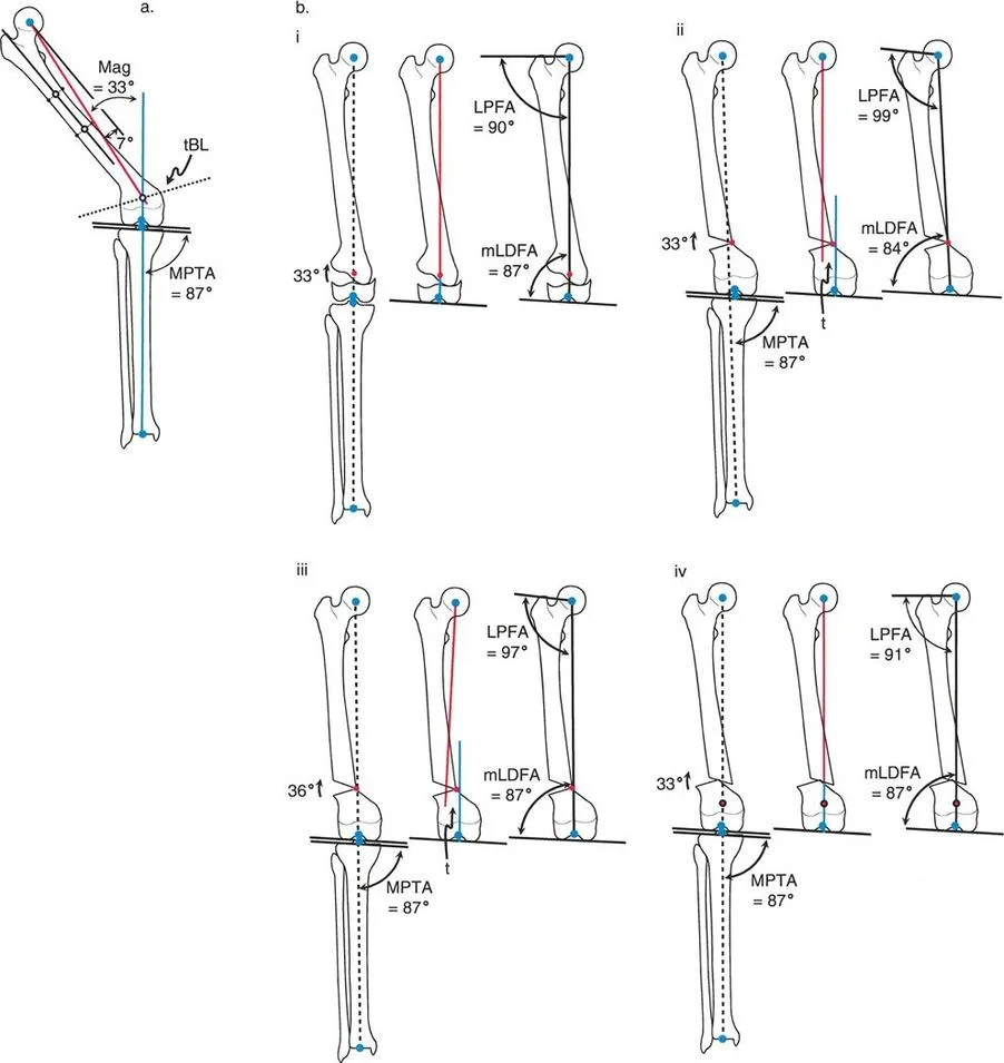
The Biomechanical Result
A secondary translational deformity is created. While the angular deformity may appear to be corrected, the mechanical axis will not be fully restored. The proximal and distal mechanical axes will be parallel but not collinear, resulting in residual Mechanical Axis Deviation (MAD).
Clinical Application
In most cases, Rule Three represents an unintended surgical error. If a surgeon ignores the CORA and simply cuts the bone where it is most convenient, hiving it at the cut site, they will create a "golf club" deformity. The joint may be parallel to the floor, but the mechanical axis will be shifted, leading to rapid joint degeneration.
However, Rule Three can be used intentionally by master surgeons to correct pre-existing translational deformities. If a bone has a pre-existing translation, applying Rule Three can create an equal and opposite translation, effectively realigning the mechanical axis.
| Paley Rule | ACA Location | Osteotomy Location | Mechanical Axis Result | Anatomic Axis Result |
|---|---|---|---|---|
| Rule 1 | At CORA | At CORA | Fully Restored (Collinear) | Perfectly Aligned (No Step-off) |
| Rule 2 | At CORA | Away from CORA | Fully Restored (Collinear) | Translated (Step-off present) |
| Rule 3 | Away from CORA | Away from CORA | Parallel but Translated (MAD) | Translated (Secondary Deformity) |
Osteotomy Sequences and Geometric Execution
Once the CORA is identified and the appropriate Paley Rule is chosen, the surgeon must select the geometry of the bone cut. Each geometry has distinct biological, biomechanical, and soft-tissue implications. The choice between opening, closing, and dome osteotomies dictates the final length of the limb and the tension on neurovascular structures.
The Opening Wedge Osteotomy Sequence
An opening wedge osteotomy involves cutting the bone and pivoting the segments open, creating a triangular void. This void is usually filled with structural bone graft (autograft or allograft) or allowed to heal via distraction osteogenesis using an external fixator.
- Biomechanics and Limb Length The opening wedge inherently lengthens the limb. The ACA is placed on the convex side of the deformity (the side that acts as the hinge).
- Soft Tissue Implications Opening a wedge tensions the soft tissues on the concave side of the deformity. Surgeons must be hyper-aware of neurovascular structures. For example, a large medial opening wedge high tibial osteotomy (HTO) can stretch the superficial medial collateral ligament and potentially tether the peroneal nerve if not carefully managed.
- Rule 2 Dynamics in Opening Wedges If the osteotomy is proximal to the CORA, and the ACA is mistakenly placed at the osteotomy level rather than the CORA, an opening wedge will leave residual MAD. To eliminate this MAD, the surgeon might be tempted to overcorrect the angle, which unfortunately alters the joint orientation, causing joint obliquity. Therefore, strict adherence to placing the ACA at the CORA is mandatory.
The Closing Wedge Osteotomy Sequence
A closing wedge osteotomy involves removing a predefined triangular wedge of bone and bringing the two flat bony surfaces together.
- Biomechanics and Limb Length The closing wedge inherently shortens the limb. The ACA is placed on the concave side of the deformity.
- Soft Tissue Implications Closing a wedge slackens the soft tissues on the convex side. This is highly advantageous when neurovascular tension is a concern, or when the patient already has a limb length discrepancy where the deformed limb is longer.
- Surgical Execution Closing wedges require precise preoperative templating. The surgeon must calculate the exact base of the wedge in millimeters to achieve the desired angular correction. Once the bone is removed, the broad cancellous surfaces provide excellent bone-to-bone contact, leading to high union rates and inherent stability, making it ideal for internal fixation with plates and screws.
The Dome Osteotomy Sequence
A dome (or focal dome) osteotomy utilizes a cylindrical or spherical cut rather than a straight transverse cut.
- Biomechanics and Limb Length The true advantage of a dome osteotomy is that it allows for pure rotation of the bone segments without altering limb length and without creating a prominent cortical step-off, even when applying Rule 2.
- Geometric Execution To execute a perfect dome osteotomy, the center of the dome's radius of curvature must be exactly at the CORA. The ACA is also placed at the CORA. As the bone segments slide along the curved cut, the mechanical axis is restored.
- Clinical Application Dome osteotomies are technically demanding and require specialized crescentic saw blades or a drill-hole technique. They are highly favored in the metaphyseal regions (like the proximal tibia or distal femur) where maintaining maximum bone contact and avoiding limb shortening is paramount.
Step by Step Guide to Frontal Plane Deformity Planning
Mastering Paley's principles requires a systematic approach to preoperative planning. Skipping steps or relying on intraoperative "eyeballing" guarantees failure.
Preoperative Radiographic Assessment
- Obtain Proper Imaging The foundation of planning is a high-quality, standing, full-length AP radiograph of both lower extremities.
- Patella Forward Positioning The radiograph must be taken with the patella facing strictly forward, regardless of foot position. This isolates the frontal plane deformity from any rotational deformity.
- Calibrate the Image Ensure the digital radiograph is calibrated using a scaling marker to allow for accurate millimeter measurements.
Executing the Preoperative Plan
- Perform the Malalignment Test Draw the mechanical axis from the center of the femoral head to the center of the ankle. Measure the MAD. Determine if the mechanical axis falls in the medial, lateral, or central zone of the knee.
- Perform the Malorientation Test Draw the individual mechanical axes of the femur and tibia. Measure the mLDFA, MPTA, LPFA, and mLDTA. Compare these to normal values to isolate the source bone of the deformity.
- Locate the CORA Draw the Proximal Mechanical Axis (PMA) and Distal Mechanical Axis (DMA) using the normal joint orientation angles. Mark their intersection as the CORA.
- Select the Osteotomy Rule Determine if the bone can be safely cut at the CORA (Rule 1) or if the cut must be moved to the metaphysis (Rule 2).
- Choose the Osteotomy Sequence Decide between an opening wedge, closing wedge, or dome based on limb length discrepancy and soft tissue constraints.
- Simulate the Correction Using digital templating software, digitally cut the bone, place the ACA, and rotate the segment. Verify that the final mechanical axis passes through the center of the knee and that joint lines are parallel to the floor.
Advanced Clinical Applications and Surgical Pearls
Applying these geometric concepts in the operating room requires bridging the gap between mathematical theory and biological reality.
Juxta Articular Deformities
Deformities located very close to the joint line present a unique challenge. The CORA is often located within the epiphysis or the joint space itself.
- Surgical Pearl You cannot cut through the CORA in these cases. You must utilize Paley's Rule 2. Place your hinge (ACA) at the joint line (the CORA), and perform your osteotomy in the metaphyseal bone.
- Managing Translation Be prepared for the resulting translation. When using a plate for fixation, you may need to use a specialized offset plate or manually contour the plate to accommodate the step-off. If using an intramedullary nail, blocking screws (Poller screws) are essential to guide the nail and maintain the translation without allowing the bone to slide back into deformity.
Diaphyseal Deformities
Midshaft deformities are typically the most straightforward to plan but can be challenging to fixate if the bone quality is poor.
* Surgical Pearl Always aim for Rule 1. Cut exactly at the CORA. This allows for the use of an intramedullary nail, which provides load-sharing biomechanics and allows for early weight-bearing.
* Beware the Sagittal Plane Diaphyseal deformities rarely exist purely in the frontal plane. Always evaluate the lateral radiograph for procurvatum or recurvatum and plan for a multi-planar correction.
Multi Apical Deformities
Some bones, particularly those affected by metabolic bone disease (like Paget's or Osteogenesis Imperfecta) or complex trauma, will have multiple bends.
* Surgical Pearl A multi-apical deformity will have multiple CORAs. You must draw the PMA, an intermediate mechanical axis, and the DMA.
* Correction Strategy You can either perform multiple osteotomies (one at each CORA) or find a single "compromise CORA" that allows for a single cut. However, a single cut for a multi-apical deformity will almost always invoke Rule 3 and create significant translation, which may be cosmetically unacceptable or biomechanically unstable.
Key Takeaways for the Deformity Surgeon
- Respect the JLCA: A widened joint line congruency angle will fool you. Always calculate your correction based on the bony geometry, but account for ligamentous laxity, or your postoperative mechanical axis will be off.
- Hinge Placement is Everything: The osteotomy cut simply allows the bone to move. The placement of the ACA dictates how it moves. Misplacing the ACA by even a few millimeters can induce unwanted translation or length changes.
- Plan for the Soft Tissues: Bones heal predictably; soft tissues do not. Always assess the peroneal nerve in severe valgus corrections and the vascular bundle in severe varus/extension corrections. Prophylactic nerve decompressions should be considered in large angular corrections.
By rigorously adhering to Dr. Dror Paley's principles, orthopedic surgeons can eliminate the guesswork from deformity correction. Transitioning from an "intuitive art" to a mathematically driven science ensures that every osteotomy restores the mechanical axis, optimizes joint loading, and provides the patient with a durable, functional limb for life.
!!! info "Academic Resource & Medical Review"
This academic resource was prepared and medically reviewed by Prof. Dr. Mohammed Hutaif, Consultant Orthopedic & Spine Surgeon. It is formulated specifically for medical students, orthopedic residents, and surgeons preparing for high-stakes board examinations (AAOS, FRCS Tr & Orth, Arab Board).
!!! warning "Disclaimer"
The surgical techniques, classifications, and clinical guidelines presented herein are for educational and academic review purposes only. They are not intended to replace institutional protocols or independent clinical judgment.
You Might Also Like