
Introduction: The Genesis of Modern Deformity Correction
The treatment of skeletal deformities has challenged orthopaedic surgeons since the dawn of the specialty—a field literally named by Nicholas Andry in 1741 from the Greek words orthos (straight) and paedis (child). For centuries, deformity correction was more art than science. Surgeons relied on "eyeball estimation," taking a wedge of bone here or there, and hoping the final radiograph looked acceptable or that the bone would magically "remodel."
While brilliant minds like Friedrich Pauwels and Gavril Ilizarov made monumental leaps in biomechanics and tissue regeneration, the global orthopaedic community still lacked a unified, standardized language. Preoperative planning was a Tower of Babel, filled with confusing terminology and inconsistent methodologies.
This all changed with the codification of Paley's Principles of Deformity Correction. Dr. Dror Paley, alongside Dr. John E. Herzenberg, transformed the "spark" of Ilizarov’s methods into a raging fire of geometric precision. By developing the CORA (Center of Rotation of Angulation) method and standardizing joint orientation nomenclature, they created a universal system that requires minimal memorization but delivers maximum surgical accuracy.
Drs. Dror Paley, MD, FRCSC, and John E. Herzenberg, MD, FRCSC, the pioneers who standardized the modern principles of deformity correction.
This masterclass dives deep into the foundational concepts of Chapter 1 of Paley's seminal text. Whether you are utilizing plates, intramedullary nails, or complex external fixators, these geometric principles remain the absolute bedrock of orthopaedic deformity correction.
The Philosophy of Principle-Based Orthopaedics
Surgical techniques and hardware devices are transient. The plates, rods, and external fixators we use today will inevitably be replaced by the innovations of tomorrow. However, the principles of geometry and biomechanics are eternal.
Paley's Principles of Deformity Correction is not a technique-centric manual; it is a principle-based system. It teaches surgeons how to analyze, understand, and quantify a deformity before ever picking up a scalpel. The method is mercifully low-tech—requiring only a radiograph, a pencil, a ruler, and a goniometer—yet it forms the foundation for even the most advanced, computer-dependent mathematical modeling of six-axis deformity correction.
The Ilizarov Hinge and the Birth of CORA
Interestingly, the CORA method began simply as an attempt to make sense of the Ilizarov apparatus. When Dr. Paley first introduced Ilizarov's methods to North America, he struggled to understand the exact placement of the Ilizarov hinge. Mismatching the location of the hinge and the actual apex of the deformity led to unwanted secondary deformities (translation). In his effort to accurately identify the perfect level for the hinge, Paley derived the CORA method. He quickly realized that these osteotomy rules were not unique to circular frames, but universally applicable to any osteotomy, from the hip to the foot.
Deconstructing the Lower Extremity: The Blueprint of Alignment
To correct a deformity, you must first be able to define normal alignment. This requires translating the complex, three-dimensional human form into simplified, two-dimensional mechanical lines and angles.
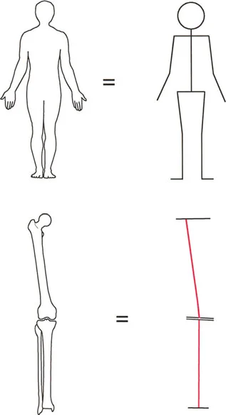
Simplifying the human form: The foundation of deformity analysis relies on reducing complex anatomical structures into mechanical lines and axes to accurately measure deviations.
Mechanical Axis vs. Anatomic Axis
The cornerstone of deformity analysis is the distinction between the mechanical and anatomic axes of the long bones. Understanding how these lines interact is non-negotiable for preoperative planning.
The Mechanical Axis:
The mechanical axis of a bone is the straight line connecting the center points of its proximal and distal joints.
* Femur: A line drawn from the center of the femoral head to the center of the knee joint.
* Tibia: A line drawn from the center of the knee joint to the center of the ankle joint.
* Lower Limb Mechanical Axis: A line drawn from the center of the femoral head directly to the center of the ankle joint. In a normally aligned limb, this line passes just medial to the center of the knee joint (Mechanical Axis Deviation or MAD).
The Anatomic Axis:
The anatomic axis is the mid-diaphyseal line of the bone.
* Femur: A line drawn through the center of the femoral diaphysis. Because the femur has an anterior bow, the anatomic axis is a curved line in the sagittal plane, but in the coronal plane, it is represented as a straight line.
* Tibia: A line drawn through the center of the tibial diaphysis.
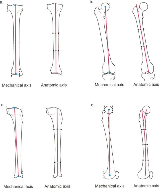
Comparison of Mechanical and Anatomic Axes in the Tibia and Femur. Note how the mechanical and anatomic axes of the tibia are nearly collinear, whereas they diverge significantly in the femur.
The Anatomic-Mechanical Angle (AMA)
In the tibia, the mechanical and anatomic axes are essentially parallel and collinear (they are the same line for practical planning purposes). However, in the femur, the mechanical axis and anatomic axis diverge.
The angle formed between the mechanical axis of the femur and the anatomic axis of the femur is known as the Anatomic-Mechanical Angle (AMA). In a normal adult, this angle is consistently 7° ± 2°. This is a critical value when planning distal femoral osteotomies or total knee arthroplasties, as it dictates the difference between anatomic and mechanical cuts.
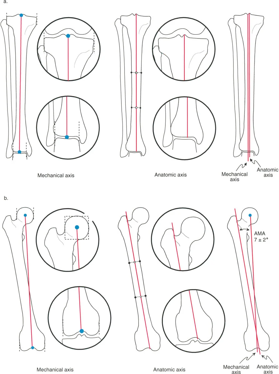
Detailed view of the Anatomic-Mechanical Angle (AMA) of the femur, demonstrating the 7° ± 2° divergence between the mechanical axis (connecting joint centers) and the anatomic axis (mid-diaphyseal line).
Defining Joint Centers and Lines
You cannot draw an axis without knowing exactly where the joints begin and end. Paley standardized the radiographic landmarks for defining joint centers, removing the guesswork from preoperative templating.
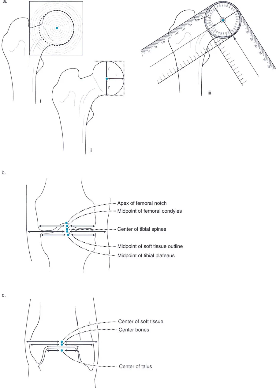
Precise radiographic landmarks for determining the center of rotation of the hip, the joint line of the knee, and the center of the ankle.
Identifying Joint Centers
- Hip Center: The center of the femoral head. This is found by placing a concentric circle template over the femoral head on an AP radiograph.
- Knee Center: The midpoint of the knee joint line. This is typically located between the tibial spines, directly inferior to the apex of the femoral intercondylar notch.
- Ankle Center: The midpoint of the width of the talar dome.
Joint Orientation Lines
Once the joint centers are established, we must define the orientation of the joints relative to the mechanical and anatomic axes.
* Proximal Femoral Line: A line drawn from the tip of the greater trochanter to the center of the femoral head.
* Distal Femoral Line: A line tangent to the most distal points of the medial and lateral femoral condyles.
* Proximal Tibial Line: A line tangent to the subchondral bone of the medial and lateral tibial plateaus (ignoring the tibial spines).
* Distal Tibial Line: A line tangent to the flat subchondral surface of the tibial plafond.
The Universal Language of Joint Orientation Angles
Before Paley's nomenclature, surgeons used a confusing array of terms to describe alignment. Paley introduced a standardized naming convention that is logical and requires little memorization. Every angle is defined by four parameters:
1. m or a: Mechanical or Anatomic axis.
2. M or L: Medial or Lateral side of the joint.
3. P or D: Proximal or Distal end of the bone.
4. F or T: Femur or Tibia.
5. A: Angle.
High-Yield Normal Values for the Lower Extremity
To accurately diagnose a deformity, you must commit these normal coronal plane values to memory:
| Angle | Acronym | Normal Value | Range |
|---|---|---|---|
| Mechanical Lateral Distal Femoral Angle | mLDFA | 87° | 85° - 90° |
| Mechanical Proximal Tibial Angle | MPTA | 87° | 85° - 90° |
| Lateral Distal Tibial Angle | LDTA | 89° | 86° - 92° |
| Mechanical Lateral Proximal Femoral Angle | mLPFA | 90° | 85° - 95° |
| Joint Line Congruency Angle | JLCA | 0° - 2° | N/A |
Surgical Pearl: Notice that the mLDFA and MPTA are both normally 87°. This means the knee joint line is not perfectly horizontal to the mechanical axis; it has a slight 3° varus tilt. However, because both angles are 87°, the joint lines of the femur and tibia remain perfectly parallel to each other (JLCA = 0°).
The Malalignment Test and Mechanical Axis Deviation (MAD)
When a patient presents with a crooked limb, the first step is to perform the Malalignment Test. This determines whether the deformity is located in the femur, the tibia, or the knee joint itself.
- Obtain a standing, full-length AP radiograph of the lower extremities.
- Draw the Mechanical Axis of the Lower Limb (a line from the center of the femoral head to the center of the ankle).
- Evaluate the Mechanical Axis Deviation (MAD). In a normal limb, this line should pass slightly medial (0 to 8 mm) to the center of the knee joint.
- If the line passes far medial to the knee center, the patient has a Varus deformity.
- If the line passes lateral to the knee center, the patient has a Valgus deformity.
- Once MAD is identified, measure the mLDFA, MPTA, and JLCA to isolate the source.
- Abnormal mLDFA = Femoral deformity.
- Abnormal MPTA = Tibial deformity.
- Abnormal JLCA = Intra-articular deformity (e.g., ligamentous laxity or cartilage loss).
The Masterclass: The CORA Method
The absolute heart of Paley's Principles of Deformity Correction is the CORA (Center of Rotation of Angulation) method. This is the universal system used to plan the exact location and geometry of a corrective osteotomy.
What is the CORA?
When a bone is bent, it consists of a proximal segment and a distal segment. If you draw the mechanical (or anatomic) axis of the proximal segment and the mechanical (or anatomic) axis of the distal segment, the point where these two lines intersect is the CORA.
The CORA represents the apex of the deformity. It is the geometric hinge point around which the distal bone segment must be rotated to restore perfect alignment.
Finding the CORA: Step-by-Step
- Draw the Proximal Axis: Using the normal joint orientation angle (e.g., an mLDFA of 87°), draw the normal mechanical axis line extending down from the proximal joint.
- Draw the Distal Axis: Using the normal joint orientation angle (e.g., an MPTA of 87°), draw the normal mechanical axis line extending up from the distal joint.
- Locate the Intersection: The exact point where these two lines cross is the CORA.
- Draw the Bisector Line: Draw a line that perfectly bisects the obtuse and acute angles formed by the intersecting axes. This bisector line is the transverse plane on which the deformity exists.
The Three Rules of Osteotomy
Identifying the CORA is only half the battle. The surgeon must now decide where to make the bone cut (the osteotomy) and where to place the mechanical hinge (the axis of correction). Paley codified this into three unbreakable geometric rules.
Rule 1: Pure Angulation
- The Rule: If the osteotomy and the hinge are both placed exactly at the CORA, the deformity will correct with pure angulation.
- The Result: The bone ends will angulate without any translation (shifting). The mechanical axis is perfectly restored.
- Clinical Application: This is the ideal scenario for most diaphyseal deformities. A closing wedge, opening wedge, or dome osteotomy performed at the CORA will yield a perfectly straight bone.
Rule 2: Angulation with Translation
- The Rule: If the hinge is placed at the CORA, but the osteotomy is performed at a different level (away from the CORA), the deformity will correct with both angulation and translation.
- The Result: The mechanical axis will be perfectly restored, but the bone ends at the osteotomy site will be translated (offset) relative to each other.
- Clinical Application: This is often done intentionally. For example, if a CORA is located very close to a joint line where there is inadequate bone stock for fixation, the surgeon can place the hinge at the CORA but make the osteotomy further down the diaphysis. The resulting translation is geometrically necessary to restore the overall mechanical axis.
Rule 3: The Danger Zone (Secondary Deformity)
- The Rule: If the osteotomy and the hinge are both placed away from the CORA, the original deformity will be corrected, but a new, secondary translation deformity will be created.
- The Result: The mechanical axis of the proximal and distal segments will be parallel, but they will not be collinear. The overall mechanical axis of the limb remains deviated.
- Clinical Application: This is the classic error made when a surgeon "eyeballs" an osteotomy without preoperative planning. Mismatching the hinge and the CORA results in a zigzag deformity. This is exactly what Dr. Paley observed in early Ilizarov frame applications, prompting the creation of the CORA method.
Advanced Applications: Scaling the Principles
The beauty of the CORA method is its scalability. While Chapter 1 introduces the foundational geometry of single-plane deformities, these exact same principles are the building blocks for correcting the most complex, multi-planar deformities seen in orthopaedics.
As outlined in the broader scope of Paley's text, these principles directly feed into advanced topics:
12 Six-Axis Deformity Analysis and Correction ... 411
16 Realignment for Mono-compartment Osteoarthritis of the Knee ... 479
Six-Axis Deformity Analysis
Deformities rarely exist in just the coronal plane. They are often combinations of angulation, translation, and rotation across the coronal, sagittal, and axial planes—a true six-axis deformity. Modern technologies, such as the Taylor Spatial Frame (TSF) and computer-assisted hexapod circular fixators, rely entirely on the surgeon's ability to accurately define the CORA. The computer software cannot fix the bone; it merely executes the geometric parameters inputted by the surgeon based on Paley's principles.
Realignment for Mono-Compartment Osteoarthritis
In cases of unicompartmental knee osteoarthritis, the cartilage loss creates an intra-articular deformity (abnormal JLCA), which drives the mechanical axis through the diseased compartment, accelerating the destruction. By applying the CORA method, surgeons can plan precise High Tibial Osteotomies (HTO) or Distal Femoral Osteotomies (DFO) to intentionally shift the mechanical axis into the healthy compartment, delaying or preventing the need for total joint arthroplasty.
Hardware Agnosticism: The Ultimate Surgical Truth
A common misconception among surgical trainees is that deformity correction is synonymous with external fixation. This is false.
The general principle of Paley's masterclass is to first analyze, understand, and quantify the deformity. Only after the geometry is solved should the surgeon begin to plan the surgical method and approach.
Regardless of which type or brand of fixation is selected, the basic principles of deformity analysis and planning are identical.
* Plates and Screws: A closing wedge osteotomy fixed with a locking plate must obey Rule 1 or Rule 2.
* Intramedullary Nails: Correcting a deformity over an IM nail often requires blocking screws (Poller screws) to force the nail to act as a hinge at the CORA.
* External Fixators: Circular frames allow for gradual correction, but the hinges must still be mathematically aligned with the CORA to prevent joint stiffness and secondary translation.
Failure to observe these principles results in less-than-perfect alignment and secondary deformities that are exponentially more difficult to correct than the original pathology. Ultimately, the surgeon must decide which device works best in their hands, but the first step of preoperative planning is universally required.
Conclusion: A Legacy of Precision
Dr. Dror Paley’s Principles of Deformity Correction is not just a textbook; it is a paradigm shift. By moving the specialty away from artistic estimation and grounding it in rigorous, reproducible geometry, Paley and Herzenberg elevated the standard of care for patients worldwide.
For the surgeon-in-training, mastering the mechanical axis, joint orientation angles, and the CORA method is not optional—it is the very definition of surgical competence in adult and pediatric orthopaedics. As hardware continues to evolve and computer navigation becomes ubiquitous, the surgeon who understands the underlying geometry will always remain the master of the operation.
Detailed Chapters & Topics
Dive deeper into specialized chapters regarding principles-of-deformity-correction-the-ultimate-guide