Radiographic Assessment of Lower Limb Deformities: The Ultimate Paley Method Masterclass
Key Takeaway
The Paley Method for lower limb deformity correction relies on meticulous radiographic assessment to quantify malalignment. By calculating the Mechanical Axis Deviation (MAD) and Joint Orientation Angles, surgeons can pinpoint the Center of Rotation of Angulation (CORA) to execute precise, biomechanically sound osteotomies.
The Foundation of Deformity Correction and Precision in Radiography
In the complex and exacting realm of orthopedic surgery, the successful correction of lower limb deformities represents the perfect marriage between biomechanical engineering and biological healing. The foundational step before a scalpel ever touches skin, before an external fixator is assembled, and before an osteotomy is planned is the meticulous, standardized radiographic assessment of the lower limb. A single millimeter or degree of error on a preoperative template can translate to catastrophic joint failure, altered kinematics, and severe patient morbidity a decade later.
Pioneered and popularized by Dr Dror Paley, the systematic approach to deformity analysis relies on a universal language of axes, angles, and rotational centers. This framework allows surgeons to quantify malalignment, pinpoint the exact apex of a deformity, and execute corrections that restore normal joint kinematics and load-bearing profiles. Prior to the widespread adoption of the Paley method, deformity correction was largely an intuitive art, prone to subjective errors and irreproducible results. Today, it is an exact science.
This masterclass provides an exhaustive, step-by-step deep dive into the radiographic assessment of lower limb deformities. We will explore the critical importance of standardized imaging, the differentiation between mechanical and anatomic axes, the calculation of joint orientation angles, and the integration of specialized views to ensure three-dimensional surgical mastery. For the surgeon-in-training, mastering these principles is not optional. It is the absolute prerequisite for safe and effective deformity correction, joint preservation, and limb lengthening procedures.
Standardized Radiographic Acquisition The Patella Forward Principle
A deformity analysis is only as accurate as the radiograph from which it is derived. Poorly positioned, non-weight-bearing, or rotated films will artificially distort joint orientation angles, mask true deformities, create pseudo-deformities, and ultimately lead to catastrophic surgical miscalculations. Precise positioning is non-negotiable for reliable surgical planning.
The Standing Long Leg Radiograph
The gold standard for coronal plane assessment is the standing anteroposterior radiograph of both lower extremities. This film must capture the entire kinetic chain from the iliac crests to the bottom of the feet.
The most critical parameter for this view is the Patella Forward position. Because the lower limb is a multi-segmental linkage system, rotation at the hip or ankle can masquerade as coronal plane deformity if the knee is not strictly standardized.
- The patient must stand with their weight evenly distributed across both lower extremities to simulate the true dynamic load on the joints.
- The patellae must be facing absolutely straight forward, regardless of where the feet point. If the patient has severe tibial torsion, the feet may point inward or outward, but the patella must remain the orienting landmark for the knee.
- If the patella is rotated, the posterior femoral condyles will not be parallel to the film cassette, artificially altering the measurement of the Mechanical Lateral Distal Femoral Angle.
- The x-ray beam should be centered at the level of the knee joint from a distance of at least ten feet to minimize magnification error and parallax distortion.
- A radiopaque magnification marker, typically a 25mm or 50mm calibration sphere, must be placed at the level of the bone to calibrate digital templating software accurately.
Leg Length Discrepancy Compensation
If the patient has a known or suspected leg length discrepancy, they must be leveled using calibrated wooden blocks under the shorter limb until the pelvis is clinically level. This is assessed by palpating the anterior superior iliac spines and ensuring they are parallel to the floor. The exact height of the block used must be recorded directly on the radiograph. Failing to level the pelvis can alter the mechanical axis due to compensatory abduction or adduction at the hip, skewing the entire mechanical axis deviation calculation and leading to inappropriate surgical interventions.
Sagittal Plane and Specialized Hindfoot Views
Coronal alignment is only one piece of the puzzle. Comprehensive assessment requires orthogonal imaging to appreciate the three-dimensional nature of the deformity.
- Standing Lateral Radiograph Taken with the knees fully extended or maximally extended if a flexion contracture exists. The film should capture the hip to the ankle. This is essential for assessing procurvatum and recurvatum deformities.
- Saltzman and Cobey Hindfoot Views Deformities of the tibia profoundly affect the foot and ankle, and vice versa. Specialized posterior roentgenograms of the foot are utilized to assess hindfoot alignment. These views are mandatory to determine if a hindfoot deformity is primary or compensatory to a proximal tibial deformity.
Defining the Axes of the Lower Extremity
To navigate Paley principles, a surgeon must master the distinction between the mechanical and anatomic axes of the lower extremity. These axes dictate how forces are transmitted across the joints during the gait cycle and serve as the foundation for all angular measurements.
The Mechanical Axis
The mechanical axis of a bone is a straight line connecting the center points of its proximal and distal joints. It represents the true line of weight-bearing force traversing the bone.
- Mechanical Axis of the Femur A line drawn from the center of the femoral head to the center of the knee joint. The center of the knee joint is specifically defined as the midpoint between the medial and lateral tibial spines, or the center of the femoral notch.
- Mechanical Axis of the Tibia A line drawn from the center of the knee joint to the center of the ankle joint, defined as the midpoint of the talar dome.
- Mechanical Axis of the Lower Limb A single line connecting the center of the femoral head directly to the center of the ankle joint. In a normal, well-aligned lower extremity, this line should pass slightly medial to the exact center of the knee joint.
The Anatomic Axis
The anatomic axis represents the mid-diaphyseal line of the bone. It is determined by drawing a line through the center points of the medullary canal at various levels of the diaphysis.
- Anatomic Axis of the Femur This line follows the medullary canal of the femur. Due to the natural offset of the femoral head and neck, the anatomic axis of the femur does not perfectly align with its mechanical axis. In a normal femur, there is a divergence of approximately seven degrees between the mechanical and anatomic axes.
- Anatomic Axis of the Tibia Unlike the femur, the anatomic axis of the tibia is essentially parallel and collinear with its mechanical axis. The mid-diaphyseal line of the tibia connects directly from the center of the knee to the center of the ankle.
Mechanical Axis Deviation and Joint Orientation Angles
The core of the Paley method relies on quantifying exactly how far a limb deviates from normal alignment and identifying which specific bone segment is responsible for that deviation.
Calculating Mechanical Axis Deviation
Mechanical Axis Deviation is the absolute distance, measured in millimeters, between the mechanical axis of the lower limb and the center of the knee joint.
To calculate Mechanical Axis Deviation, the surgeon draws a line from the center of the femoral head to the center of the ankle joint. In a normal limb, this line passes 8 millimeters to 10 millimeters medial to the center of the knee joint.
* If the line passes further medial than normal, or entirely medial to the medial tibial plateau, the patient has a varus deformity.
* If the line passes lateral to the center of the knee joint, the patient has a valgus deformity.
Identifying an abnormal Mechanical Axis Deviation is the trigger that initiates the rest of the deformity analysis. It tells the surgeon that a deformity exists, but it does not tell them where the deformity is located. To find the source, the surgeon must measure the joint orientation angles.
Femoral and Tibial Joint Orientation Angles
Joint orientation angles describe the relationship between the mechanical or anatomic axis of a bone and its articular surface. Dr Paley standardized the nomenclature for these angles, utilizing a four-letter acronym system.
The first letter denotes Mechanical (m) or Anatomic (a). The second letter denotes Medial (M) or Lateral (L). The third letter denotes Proximal (P) or Distal (D). The fourth letter denotes Femoral (F) or Tibial (T) Angle (A).
| Angle Acronym | Full Name | Normal Value | Clinical Significance |
|---|---|---|---|
| mLDFA | Mechanical Lateral Distal Femoral Angle | 87° (85°-90°) | Determines coronal plane deformity in the distal femur. |
| MPTA | Medial Proximal Tibial Angle | 87° (85°-90°) | Determines coronal plane deformity in the proximal tibia. |
| LPFA | Lateral Proximal Femoral Angle | 90° (85°-95°) | Evaluates the relationship of the greater trochanter to the femoral head. |
| LDTA | Lateral Distal Tibial Angle | 89° (86°-92°) | Determines coronal plane deformity of the ankle mortise. |
| aLDFA | Anatomic Lateral Distal Femoral Angle | 81° (79°-83°) | Used when templating with intramedullary devices based on the anatomic axis. |
The Joint Line Congruency Angle
The Joint Line Congruency Angle measures the orientation of the distal femoral articular line relative to the proximal tibial articular line. In a normal knee, these two lines are nearly parallel, resulting in a Joint Line Congruency Angle of 0 to 2 degrees.
An abnormal Joint Line Congruency Angle indicates intra-articular deformity, ligamentous laxity, or cartilage loss. A surgeon must carefully evaluate this angle, as correcting a purely extra-articular bony deformity without accounting for severe ligamentous laxity will result in residual Mechanical Axis Deviation.
The Center of Rotation of Angulation
Once an abnormal joint orientation angle is identified, the surgeon knows which bone is deformed. The next critical step is determining the exact apex of that deformity. This apex is known as the Center of Rotation of Angulation.
Defining the CORA
The Center of Rotation of Angulation is the point at which the proximal mechanical axis line and the distal mechanical axis line of a deformed bone intersect.
To find the CORA, the surgeon must draw the normal mechanical axis line for the proximal segment of the bone and the normal mechanical axis line for the distal segment of the bone. Because the bone is deformed, these two lines will not be collinear. Instead, they will intersect at a specific point. This intersection point is the CORA.
The angle formed by the intersection of these two lines represents the true magnitude of the deformity. The bisector of this angle is known as the bisector line, which plays a critical role in determining the axis of correction during surgery.
Multiple CORA Deformities
In complex cases, a bone may have more than one deformity, such as a midshaft fracture malunion combined with a distal metaphyseal bowing. In these instances, drawing the proximal and distal mechanical axes will not accurately describe the deformity because the middle segment of the bone is also malaligned.
Surgeons must utilize the mid-diaphyseal line of the intermediate segment to identify multiple CORAs. The proximal axis will intersect the intermediate axis to form the first CORA, and the intermediate axis will intersect the distal axis to form the second CORA. Recognizing multiple CORAs is essential, as ignoring one will lead to a secondary translation deformity during correction.
The Three Osteotomy Rules of Dr Dror Paley
Identifying the CORA is only half the battle. The surgeon must then decide where to cut the bone (the osteotomy) and where to place the hinge or rotational center of the fixation device (the Axis of Correction of Angulation). Dr Paley formulated three fundamental osteotomy rules that dictate the geometric outcomes of deformity correction. Mastering these rules is the hallmark of an advanced deformity surgeon.
Osteotomy Rule One
The Rule When the osteotomy and the Axis of Correction of Angulation both pass through the CORA, the deformity corrects by pure angulation without any translation.
Clinical Application This is the most biomechanically sound and anatomically perfect correction. The bone ends simply hinge open or closed at the apex of the deformity. The mechanical axis is perfectly restored, and the local bone anatomy remains collinear. This rule is highly favored when the CORA is located in the metaphysis or diaphysis where a cut is surgically feasible and safe.
Osteotomy Rule Two
The Rule When the Axis of Correction of Angulation passes through the CORA, but the osteotomy is performed at a different level, the deformity corrects by angulation combined with translation.
Clinical Application Sometimes, the CORA is located precisely at the joint line or in an area of poor bone stock where an osteotomy is impossible or unsafe. In this scenario, the surgeon places the hinge of the external fixator exactly at the CORA but cuts the bone at a safe distance away (e.g., in the metaphysis). As the hinge opens, the bone will simultaneously angulate and translate. This translation is not a complication. It is a necessary geometric requirement to perfectly realign the proximal and distal mechanical axes.
Osteotomy Rule Three
The Rule When the osteotomy and the Axis of Correction of Angulation are both located outside the CORA, the deformity corrects by angulation, but a secondary translation deformity is created.
Clinical Application This rule represents a geometric error that surgeons must actively avoid or consciously utilize for specific complex corrections. If a surgeon places the hinge away from the CORA and cuts the bone away from the CORA, the mechanical axis will not be restored to a straight line. Instead, a zigzag deformity is created. The mechanical axis is translated, resulting in shear forces across the joint. Rule Three is generally considered a pitfall in standard deformity correction unless the surgeon is intentionally trying to translate the mechanical axis to offload a specific arthritic compartment.
Step by Step Radiographic Deformity Analysis
To synthesize these principles, surgeons employ a standardized algorithm for every patient. This ensures no subtle deformity is missed and prevents the catastrophic error of operating on the wrong bone segment.
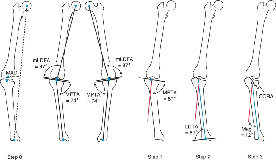
Step One Identifying the Deformity
The surgeon begins with the Malalignment Test. Using the 51-inch standing radiograph, the mechanical axis of the lower extremity is drawn from the center of the femoral head to the center of the ankle. The Mechanical Axis Deviation is measured.
* If the Mechanical Axis Deviation is within normal limits (0 to 10 millimeters medial), coronal alignment is normal.
* If the Mechanical Axis Deviation is abnormal, the surgeon proceeds to Step Two to locate the source of the malalignment.
Step Two Joint Angle Measurement
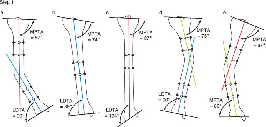
This is known as the Malorientation Test. The surgeon systematically measures the mLDFA, MPTA, LDTA, and Joint Line Congruency Angle.
* Compare the patient's measured angles against the standard normal values.
* If the mLDFA is 95 degrees (normal is 87), the femur has a varus deformity.
* If the MPTA is 80 degrees (normal is 87), the tibia has a varus deformity.
* If both are abnormal, a multi-apical or multi-segmental deformity exists.
Step Three CORA Localization
Focusing on the deformed bone, the surgeon draws the proximal mechanical axis line and the distal mechanical axis line.
* The proximal line is drawn starting from the center of the proximal joint, at the normal joint orientation angle.
* The distal line is drawn starting from the center of the distal joint, at the normal joint orientation angle.
* The intersection of these two lines identifies the CORA. The angle between them dictates the degrees of correction required.
Step Four Osteotomy Planning
With the CORA identified, the surgeon applies Paley's Osteotomy Rules.
* Determine if the bone quality and soft tissue envelope at the CORA permit a safe osteotomy.
* If yes, apply Rule One. Plan the cut and the hinge at the CORA.
* If no, apply Rule Two. Plan the cut at a safe metaphyseal location, but maintain the hinge exactly at the CORA to allow for the necessary compensatory translation.
* Calculate the required wedge size for an opening or closing wedge osteotomy, or template the spatial frame parameters for gradual correction.
Sagittal Plane Deformities and Rotational Considerations
While coronal plane deformities (varus and valgus) are the most visually apparent, lower limb deformities are inherently three-dimensional. Neglecting the sagittal and axial planes will result in severe functional deficits.
Procurvatum and Recurvatum Analysis
Sagittal plane deformities are evaluated on the standing lateral long-leg radiograph. The principles of CORA and joint orientation angles apply identically to the sagittal plane.
* Posterior Distal Femoral Angle Evaluates the sagittal alignment of the distal femur. Abnormalities here manifest as femoral procurvatum (anterior bowing) or recurvatum (posterior bowing).
* Posterior Proximal Tibial Angle Evaluates the natural posterior slope of the tibial plateau, which is typically around 81 degrees. Altering this slope during a coronal correction can severely destabilize the cruciate ligaments of the knee.
* Anterior Distal Tibial Angle Evaluates the sagittal orientation of the ankle joint.
When a deformity exists in both the coronal and sagittal planes, it is termed an oblique plane deformity. Instead of performing two separate corrections, the Paley method calculates the true oblique plane of the deformity, allowing for a single-axis correction that addresses both planes simultaneously.
Assessing Torsional Malalignment
Rotational, or torsional, deformities cannot be accurately quantified on standard radiographs. They require clinical examination (such as the thigh-foot angle or transmalleolar axis) and advanced imaging, typically a computed tomography rotational study.
Femoral anteversion and tibial torsion must be assessed independently. A common pitfall is correcting a severe varus deformity while ignoring a concomitant 30-degree internal tibial torsion. The mechanical axis may be restored on the AP radiograph, but the patient will suffer from severe in-toeing, patellofemoral maltracking, and gait dysfunction. Torsional corrections are often combined with angular corrections using a single oblique osteotomy cut or a six-axis external fixator.
Avoiding Common Pitfalls in Preoperative Planning
Even with a mastery of Paley principles, surgeons must remain vigilant against technical and conceptual errors during the planning phase.
Radiographic Magnification Errors
Digital templating software relies heavily on the accuracy of the calibration marker. If the calibration sphere is placed anterior to the bone (e.g., on top of the patella) rather than in the same coronal plane as the bone, the software will incorrectly calculate magnification. This leads to underestimating or overestimating the required wedge size in opening-wedge osteotomies, resulting in overcorrection or undercorrection. Always ensure the marker is taped to the medial or lateral aspect of the joint line.
Masked Deformities and Compensatory Mechanisms
The human body is highly adaptive. A severe varus deformity in the tibia may be partially masked by a compensatory valgus deformity in the subtalar joint. If the surgeon only assesses the knee and corrects the tibia to a neutral mechanical axis, the patient will be left with a rigid, uncompensated valgus foot, leading to severe pain and difficulty walking.
This underscores the necessity of the Paley method's holistic approach. The entire kinetic chain, from the hip down to the hindfoot, must be evaluated as a single, interconnected biomechanical linkage. By strictly adhering to standardized radiographic acquisition, meticulously calculating joint orientation angles, and faithfully applying the three osteotomy rules, the orthopedic surgeon can transform complex, intimidating deformities into predictable, highly successful surgical outcomes.
!!! info "Academic Resource & Medical Review"
This academic resource was prepared and medically reviewed by Prof. Dr. Mohammed Hutaif, Consultant Orthopedic & Spine Surgeon. It is formulated specifically for medical students, orthopedic residents, and surgeons preparing for high-stakes board examinations (AAOS, FRCS Tr & Orth, Arab Board).
!!! warning "Disclaimer"
The surgical techniques, classifications, and clinical guidelines presented herein are for educational and academic review purposes only. They are not intended to replace institutional protocols or independent clinical judgment.
You Might Also Like