Paley Principles: Mastering Lower Limb Alignment & Deformity Correction
Key Takeaway
Paley principles standardize lower limb alignment and joint orientation, defining mechanical/anatomic axes and Mechanical Axis Deviation (MAD). Essential for precise orthopedic deformity correction, they prevent premature joint degeneration and optimize surgical outcomes.
Introduction to Lower Limb Deformity Correction
The foundation of modern orthopedic deformity correction and limb lengthening rests upon a precise, mathematical understanding of normal lower limb alignment and joint orientation. Before any surgeon can master the Center of Rotation of Angulation (CORA) method or execute complex osteotomies, they must first possess a flawless grasp of the normative anatomical values that dictate human biomechanics.
Historically, the orthopedic literature was plagued by inconsistent terminology. Different authors used conflicting names for the same anatomical angles, making communication, preoperative planning, and outcome comparison incredibly difficult. Dr. Dror Paley and colleagues revolutionized this field by introducing a standardized, universally applicable nomenclature system. This masterclass translates these foundational Paley principles into a high-yield, comprehensive guide designed specifically for orthopedic surgeons-in-training. We will deconstruct the mechanical and anatomic axes, decode the joint orientation nomenclature, and explore the clinical applications of these metrics in surgical planning.
Understanding these principles is not merely an academic exercise; it is the fundamental prerequisite for preventing premature joint degeneration, optimizing implant survivorship in arthroplasty, and ensuring functional restoration in post-traumatic and congenital deformities.
Defining the Axes Mechanical vs Anatomic
To understand joint orientation, we must first define the reference lines used to measure it. The distinction between the mechanical and anatomic axes is the bedrock of lower limb deformity analysis. Every preoperative plan begins with accurately drawing these lines on full-length, weight-bearing radiographs.
The Mechanical Axis
The mechanical axis of a bone is a straight line connecting the center points of its proximal and distal joints. It represents the true mechanical lever arm of the bone during weight-bearing activities.
- Femur: The mechanical axis line is drawn from the center of the femoral head to the center of the knee joint. The center of the knee joint is specifically defined as the center of the femoral notch or the midpoint between the tibial spines.
- Tibia: The mechanical axis line is drawn from the center of the tibial plateau to the center of the tibial plafond (the ankle joint).
- Lower Limb Overall: The mechanical axis of the entire lower extremity is a line connecting the center of the femoral head to the center of the ankle joint. In a normally aligned limb, this line passes just medial to the center of the knee joint.
The Anatomic Axis
The anatomic axis represents the mid-diaphyseal line of the bone. It is the line that best bisects the medullary canal.
- Femur: A line drawn through the center of the femoral diaphysis. Because the femur has a natural anterior bow in the sagittal plane and a valgus orientation in the frontal plane, its anatomic axis is distinct from its mechanical axis. The angle between the anatomic and mechanical axes of the femur (AMA) is typically between 5 and 7 degrees, depending on the width of the pelvis and the length of the femur.
- Tibia: A line drawn through the center of the tibial diaphysis. Crucially, in the tibia, the anatomic and mechanical axes are essentially parallel. For practical surgical planning purposes in the frontal plane, they are considered collinear.
Alignment vs Joint Orientation The Critical Distinction
When evaluating the frontal plane of the lower extremity, surgeons must assess two separate but highly interrelated concepts. These are Lower Limb Alignment and Joint Orientation. Conflating these two concepts is a common pitfall in early surgical training.
Lower Limb Alignment
Alignment refers to the collinearity of the hip, knee, and ankle joints. It dictates how weight-bearing forces are distributed across the articular cartilage of the knee. Global limb alignment determines the mechanical environment of the entire extremity.
Alignment is best judged using a long-standing, weight-bearing anteroposterior (AP) radiograph of the entire lower extremity. The patient must be positioned with the patellae facing strictly forward to eliminate the effects of rotation on the frontal plane projection. The primary metric for assessing global alignment is the Mechanical Axis Deviation.
Mechanical Axis Deviation MAD
Mechanical Axis Deviation (MAD) is the perpendicular distance from the mechanical axis of the entire lower limb to the center of the knee joint. It is the definitive test for global limb malalignment.
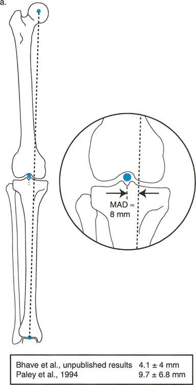
- Normal MAD: The mechanical axis normally passes slightly medial to the exact center of the knee joint. The normal MAD is approximately 8 mm (± 7 mm) medial to the center of the knee.
- Pathologic MAD: A mechanical axis passing excessively medial to the knee center indicates a varus alignment. This predisposes the patient to medial compartment osteoarthritis due to pathologic compressive forces. Conversely, a mechanical axis passing lateral to the knee center indicates a valgus alignment, predisposing the patient to lateral compartment osteoarthritis.
Joint Orientation
While alignment tells us if the limb is crooked, joint orientation tells us where and why it is crooked. Orientation refers to the position of each articular surface relative to the axes of the individual limb segments (the tibia and femur).
If a patient has an abnormal MAD, the surgeon must measure the joint orientation angles of both the femur and the tibia to determine which bone (or if both bones) is contributing to the malalignment. Correcting alignment without respecting joint orientation leads to joint line obliquity. Joint line obliquity causes sheer stress on the articular cartilage, ligamentous instability, and ultimately, premature joint failure.
Establishing Joint Orientation Lines
To measure joint orientation angles accurately, we must first draw precise joint lines in both the frontal and sagittal planes. These lines serve as the foundation for the Paley nomenclature system.
The Knee Joint Line
- Frontal Plane Distal Femur: The joint orientation of the distal femur is drawn as a straight line connecting the two most distal points of the medial and lateral femoral condyles. For pediatric patients with open physes, this line can be drawn connecting the points where the growth plate exits anteriorly and posteriorly.
- Frontal Plane Proximal Tibia: On the tibial side, the joint line connects the flat, subchondral surfaces of the medial and lateral tibial plateaus. It is crucial to exclude osteophytes when drawing this line.
- Sagittal Plane: Evaluating the distal femur in the sagittal plane can be challenging due to the curvature of the condyles. Blumensaat's line, which appears as a flat radiodense line representing the roof of the intercondylar notch, serves as an excellent surrogate for the joint orientation line of the distal femur. This is particularly useful for evaluating sagittal plane deformities (recurvatum or procurvatum) secondary to distal femoral growth arrest.
The Hip Joint Line
The hip joint presents a unique geometric challenge. In the frontal plane, the proximal femoral joint orientation line is typically drawn from the center of the femoral head to the tip of the greater trochanter. Alternatively, surgeons frequently rely on the neck-shaft angle (the angle between the anatomic axis of the femoral shaft and the axis of the femoral neck) to evaluate proximal femoral geometry.
The Ankle Joint Line
In the frontal plane, the distal tibial joint orientation line is drawn across the flat subchondral bone of the tibial plafond. In the sagittal plane, the joint line connects the most anterior and posterior points of the tibial plafond.
Paley Nomenclature and Joint Orientation Angles
Dr. Paley introduced a standardized prefix system that eliminates ambiguity in deformity planning. Every angle is defined by a specific sequence of letters that describe exactly what is being measured.
The Standardized Paley Prefix System
The nomenclature follows a strict formula: [Axis] + [Medial/Lateral] + [Proximal/Distal] + [Bone] + Angle.
- Axis: 'm' for mechanical, 'a' for anatomic.
- Side: 'M' for medial, 'L' for lateral, 'A' for anterior, 'P' for posterior.
- Location: 'P' for proximal, 'D' for distal.
- Bone: 'F' for femur, 'T' for tibia.
- Angle: Always ends with 'A' for Angle.
For example, mLDFA stands for the mechanical Lateral Distal Femoral Angle.
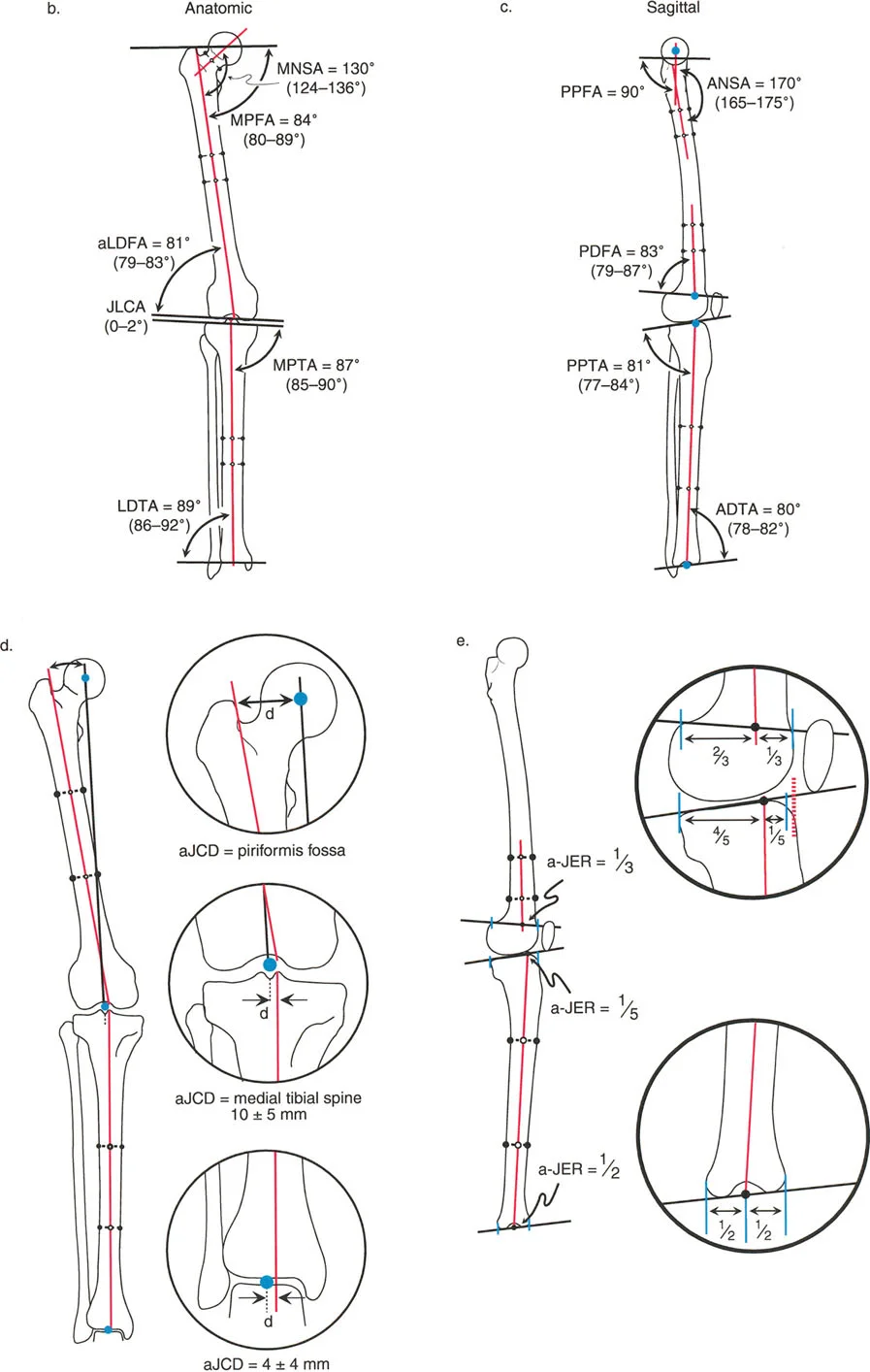
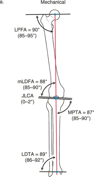
Frontal Plane Femoral Angles
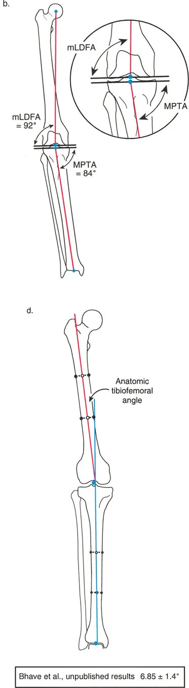
- mLDFA (mechanical Lateral Distal Femoral Angle): The angle between the mechanical axis of the femur and the distal femoral joint line on the lateral side.
- Normal Value: 87° (Range: 85° - 90°)
- aLDFA (anatomic Lateral Distal Femoral Angle): The angle between the anatomic axis of the femur and the distal femoral joint line on the lateral side.
- Normal Value: 81° (Range: 79° - 83°)
- mLPFA (mechanical Lateral Proximal Femoral Angle): The angle between the mechanical axis of the femur and the proximal femoral joint line.
- Normal Value: 90° (Range: 85° - 95°)
Frontal Plane Tibial Angles
Because the mechanical and anatomic axes of the tibia are parallel, we generally refer only to the mechanical angles, which apply to both axes.
- MPTA (Medial Proximal Tibial Angle): The angle between the mechanical/anatomic axis of the tibia and the proximal tibial joint line on the medial side.
- Normal Value: 87° (Range: 85° - 90°)
- LDTA (Lateral Distal Tibial Angle): The angle between the mechanical/anatomic axis of the tibia and the distal tibial joint line on the lateral side.
- Normal Value: 89° (Range: 86° - 92°)
Joint Line Congruency Angle JLCA
The Joint Line Congruency Angle (JLCA) is measured between the joint line of the distal femur and the joint line of the proximal tibia. It evaluates the soft tissue envelope (ligamentous laxity) and cartilage wear of the knee.
* Normal Value: 0° to 2° (joint lines are nearly parallel).
* Clinical Significance: A JLCA greater than 2° indicates intra-articular deformity, such as collateral ligament laxity or asymmetric cartilage loss. If a patient has a varus deformity with a large JLCA, correcting only the bony deformity without addressing the ligamentous laxity will result in under-correction.
Sagittal Plane Angles
Sagittal plane analysis is equally critical, particularly for preventing recurvatum or procurvatum deformities that alter gait kinematics.
- aPDFA (anatomic Posterior Distal Femoral Angle): 83° (Range: 79° - 87°)
- PPTA (Posterior Proximal Tibial Angle): 81° (Range: 77° - 84°). This represents the natural posterior slope of the tibial plateau.
- ADTA (Anterior Distal Tibial Angle): 80° (Range: 78° - 82°).
Summary Table of Normal Joint Orientation Angles
| Angle | Description | Normal Value | Clinical Range |
|---|---|---|---|
| mLDFA | mechanical Lateral Distal Femoral Angle | 87° | 85° - 90° |
| aLDFA | anatomic Lateral Distal Femoral Angle | 81° | 79° - 83° |
| MPTA | Medial Proximal Tibial Angle | 87° | 85° - 90° |
| LDTA | Lateral Distal Tibial Angle | 89° | 86° - 92° |
| mLPFA | mechanical Lateral Proximal Femoral Angle | 90° | 85° - 95° |
| JLCA | Joint Line Congruency Angle | 0° - 2° | N/A |
| PPTA | Posterior Proximal Tibial Angle | 81° | 77° - 84° |
| ADTA | Anterior Distal Tibial Angle | 80° | 78° - 82° |
The Center of Rotation of Angulation CORA Method
Once a malorientation is identified, the surgeon must determine exactly where to perform the osteotomy. This is achieved using the Center of Rotation of Angulation (CORA) method. The CORA is the foundational geometric concept for planning angular deformity correction.
Defining the CORA
The CORA is the point where the proximal mechanical (or anatomic) axis line intersects with the distal mechanical (or anatomic) axis line of a deformed bone.
To find the CORA:
1. Draw the normal joint orientation line for the proximal segment.
2. Draw the proximal axis line at the normal normative angle (e.g., 87° for MPTA) relative to that joint line.
3. Draw the normal joint orientation line for the distal segment.
4. Draw the distal axis line at the normal normative angle relative to the distal joint line.
5. The intersection of these two axis lines is the CORA.
Identifying the Magnitude of Deformity
The angle formed by the intersection of the proximal and distal axis lines represents the true magnitude of the angular deformity. Furthermore, a line bisecting this supplementary angle is known as the bisector line. The bisector line is critical because placing a hinge on this line ensures that the bone ends will not compress or distract asymmetrically during an opening or closing wedge osteotomy.
Single vs Multi Apical Deformities
- Uni-apical Deformity: The proximal and distal axes intersect at a single point (one CORA), indicating a single apex of deformity.
- Multi-apical Deformity: The proximal and distal axes do not intersect at the site of the obvious clinical deformity, or they run parallel to each other. This indicates translation or multiple apices of deformity. In these cases, a mid-diaphyseal line must be drawn to intersect with both the proximal and distal axes, revealing two separate CORAs.
The Three Paley Osteotomy Rules
Identifying the CORA is only half the battle. The surgeon must then decide where to cut the bone (the osteotomy site) and where to pivot the bone (the Axis of Correction of Angulation, or ACA). Dr. Paley codified the geometric relationship between the CORA, the ACA, and the osteotomy site into three fundamental rules. Mastering these rules is mandatory for any deformity surgeon.
Osteotomy Rule 1 Pure Angulation
- The Rule: When the osteotomy and the ACA both pass through the CORA, the correction will result in pure angulation without translation.
- The Result: The proximal and distal mechanical axes will become perfectly collinear. The bone ends at the osteotomy site will angulate seamlessly.
- Clinical Application: This is the ideal scenario. It is frequently used in opening wedge high tibial osteotomies (HTO) or distal femoral osteotomies (DFO) where the cut is made directly through the apex of the deformity.
Osteotomy Rule 2 Angulation and Translation
- The Rule: When the ACA passes through the CORA, but the osteotomy is performed at a different level (outside the CORA), the correction will result in angulation combined with translation of the bone ends.
- The Result: The proximal and distal mechanical axes will still become perfectly collinear (which is the ultimate goal of deformity correction). However, the bone ends at the osteotomy site will offset or translate relative to each other.
- Clinical Application: This rule is utilized when the CORA is located too close to the joint line for adequate fixation. The surgeon places the hinge (ACA) at the CORA to ensure perfect mechanical axis realignment, but makes the actual bone cut further down the diaphysis to allow room for plates or external fixator pins. The surgeon must anticipate and accept the resulting diaphyseal translation.
Osteotomy Rule 3 Unintended Translation
- The Rule: When the osteotomy and the ACA are both placed outside the CORA, the correction will result in a secondary translation deformity.
- The Result: The proximal and distal mechanical axes will become parallel, but they will not be collinear. A new, iatrogenic translation deformity is created.
- Clinical Application: Rule 3 is generally a pitfall to be avoided. It occurs when a surgeon ignores the CORA and simply cuts and hinges the bone at an arbitrary location. The only exception is when a patient presents with a pre-existing translation deformity, and Rule 3 is intentionally applied in reverse to restore collinearity.
Step by Step Preoperative Planning Algorithm
Executing a flawless deformity correction requires a disciplined, step-by-step approach to preoperative planning. Surgeons should utilize the following algorithm for every case.
Step 1 The Malalignment Test
Begin with a 51-inch standing AP radiograph. Draw the mechanical axis of the entire lower limb (center of femoral head to center of ankle). Measure the Mechanical Axis Deviation (MAD).
* If the MAD is normal (8 mm medial to knee center), global alignment is normal.
* If the MAD is abnormal, proceed to Step 2.
Step 2 The Malorientation Test
If the MAD is abnormal, you must identify the source. Measure the mLDFA, MPTA, and JLCA.
* Femoral Origin: If the mLDFA is abnormal but the MPTA is normal, the deformity is in the femur.
* Tibial Origin: If the MPTA is abnormal but the mLDFA is normal, the deformity is in the tibia.
* Combined Origin: If both are abnormal, a double-level osteotomy may be required.
* Intra-articular Origin: If mLDFA and MPTA are normal but the JLCA is greater than 2°, the malalignment is driven by soft tissue laxity or cartilage loss within the knee joint.
Step 3 CORA Identification and Planning
Once the deformed bone is identified, draw the proximal and distal joint orientation lines. Project the normal mechanical axes from these lines until they intersect. This is your CORA.
Step 4 Applying the Osteotomy Rules
Decide on the surgical approach. Can you safely cut through the CORA (Rule 1)? If the CORA is intra-articular or too close to the joint, you must plan an osteotomy away from the CORA while keeping your hinge at the CORA (Rule 2), anticipating the necessary translation.
Step 5 Implant Selection and Templating
Choose the appropriate fixation device (e.g., locking plate, intramedullary nail, or circular external fixator). Template the hardware onto the planned correction to ensure adequate screw purchase in the proximal and distal segments.
High Yield Surgical Pearls for Deformity Correction
- Beware the Fibula: In tibial deformity correction, the intact fibula acts as a lateral tether. Failing to perform a fibular osteotomy or release the proximal tibiofibular joint during a large varus/valgus correction will lead to under-correction or catastrophic hardware failure.
- The Peroneal Nerve Risk: Valgus deformities of the proximal tibia stretch the common peroneal nerve. When correcting a severe valgus deformity (e.g., performing a medial closing wedge or lateral opening wedge osteotomy), prophylactic peroneal nerve decompression is highly recommended to prevent postoperative foot drop.
- Respect the Joint Line Obliquity: Never correct a femoral deformity with a tibial osteotomy, or vice versa. While this might normalize the MAD, it will severely tilt the knee joint line relative to the ground. A tilted joint line creates sheer forces that rapidly accelerate osteoarthritis. Always correct the bone that is actually deformed.
- Sagittal Plane Dominance: While frontal plane deformities (varus/valgus) are visually obvious, sagittal plane deformities (flexion/extension contractures, recurvatum) often cause more severe functional impairment and gait deviations. Always evaluate orthogonal views.
*
!!! info "Academic Resource & Medical Review"
This academic resource was prepared and medically reviewed by Prof. Dr. Mohammed Hutaif, Consultant Orthopedic & Spine Surgeon. It is formulated specifically for medical students, orthopedic residents, and surgeons preparing for high-stakes board examinations (AAOS, FRCS Tr & Orth, Arab Board).
!!! warning "Disclaimer"
The surgical techniques, classifications, and clinical guidelines presented herein are for educational and academic review purposes only. They are not intended to replace institutional protocols or independent clinical judgment.
You Might Also Like