Mastering Frontal Plane Deformity Correction: Paley Principles & Osteotomy Guide
Key Takeaway
The Paley method for frontal plane realignment osteotomy is a systematic approach to mathematically quantify and correct limb deformities. It uses biomechanics, mechanical axes, and the Center of Rotation of Angulation (CORA) to precisely plan osteotomies, restoring optimal limb function and preventing premature joint degeneration.
Introduction to Frontal Plane Realignment and Deformity Correction
In the realm of orthopedic surgery, the transition from subjectively estimating a deformity to mathematically quantifying and correcting it has fundamentally revolutionized patient outcomes. Pioneered by Dr. Dror Paley, the systematic approach to deformity correction relies on a rigorous, uncompromising understanding of biomechanics, joint orientation, and mechanical axes. For orthopedic surgeons, residents, and fellows, mastering frontal plane realignment osteotomy is not merely an academic exercise. It is the foundational skillset required to prevent premature joint degeneration, restore optimal limb function, and execute complex reconstructive procedures with pinpoint accuracy.
Historically, osteotomies were performed based on visual alignment or basic intraoperative fluoroscopy, often resulting in secondary deformities, iatrogenic translation, or failure to address the true apex of the deformity. The Paley method introduced a paradigm shift, treating the lower extremity as a precise geometric construct governed by measurable angles and axes. This comprehensive guide delves deeply into the concepts of osteotomy and frontal plane realignment. We will heavily expand upon the principles of the Center of Rotation of Angulation, Mechanical Axis Deviation, and the critical decision-making processes involved in treating complex, multiapical deformities of the femur and tibia. By internalizing these advanced concepts, the orthopedic surgeon transitions from a technician who simply cuts bone to an architect who meticulously rebuilds the lower extremity structural integrity.
The Lexicon of Deformity Paley Foundational Principles
Before attempting to plan or execute a correction for a uniapical or multiapical deformity, the orthopedic surgeon must become completely fluent in the language of limb alignment. The lower extremity is governed by strict mechanical and anatomic axes that dictate how weight-bearing load is transferred across the hip, knee, and ankle joints. Alterations in these axes lead to abnormal stress distribution, cartilage wear, and eventual osteoarthritis.
Mechanical Versus Anatomic Axes
Understanding the distinction between mechanical and anatomic axes is the first step in deformity analysis. These lines form the basis for all subsequent angular measurements.
- Mechanical Axis: This is a straight line connecting the center of the proximal joint to the center of the distal joint of a specific bone or an entire limb. In the lower extremity, the mechanical axis of the entire limb runs from the center of the femoral head to the center of the ankle plafond. In a normally aligned limb, this weight-bearing line passes slightly medial to the center of the knee joint, typically through the medial tibial spine.
- Anatomic Axis: This is a line drawn directly down the center of the medullary canal of the diaphysis of a bone. In the tibia, the mechanical and anatomic axes are nearly parallel and are often superimposed on one another for planning purposes. However, in the femur, the mechanical and anatomic axes diverge by approximately five to seven degrees due to the offset of the femoral neck and head.
Joint Orientation Angles and Normal Values
Joint orientation is evaluated by measuring the angles formed by the intersection of the mechanical or anatomic axes with the respective joint lines. Preserving or restoring these specific angles is the ultimate goal of any realignment osteotomy. A deviation from these normal values indicates a bony deformity that requires correction.
| Angle Abbreviation | Full Terminology | Normal Range | Average Value |
|---|---|---|---|
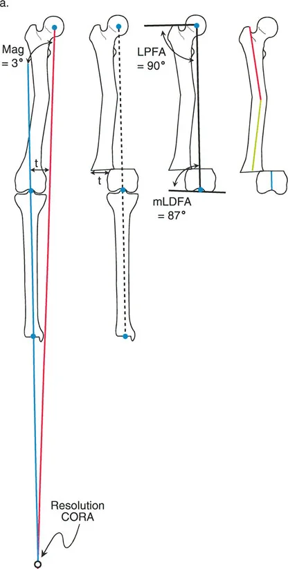
| mLDFA | Mechanical Lateral Distal Femoral Angle | 85° to 90° | 87° |
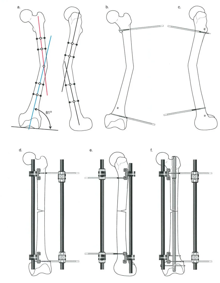
| aLDFA | Anatomic Lateral Distal Femoral Angle | 79° to 83° | 81° |
| LPFA | Lateral Proximal Femoral Angle | 85° to 95° | 90° |
| MPTA | Medial Proximal Tibial Angle | 85° to 90° | 87° |
| LDTA | Lateral Distal Tibial Angle | 86° to 92° | 89° |
| JLCA | Joint Line Convergence Angle | 0° to 2° | 1° |
Surgical Pearl: Always measure the Joint Line Convergence Angle during your preoperative planning. The JLCA represents the angle between the distal femoral articular line and the proximal tibial articular line. An abnormal JLCA indicates either intra-articular cartilage loss, ligamentous laxity, or a dynamic subluxation, which must be accounted for independently of the bony deformity.
Mechanical Axis Deviation and Joint Line Convergence Angle
Mechanical Axis Deviation is the absolute perpendicular distance from the mechanical axis of the entire limb to the center of the knee joint. It is the primary indicator of overall limb malalignment.
- Varus Deformity: A medial shift of the mechanical axis relative to the center of the knee. This overloads the medial compartment.
- Valgus Deformity: A lateral shift of the mechanical axis relative to the center of the knee. This overloads the lateral compartment.
The primary objective of frontal plane realignment is to eliminate Mechanical Axis Deviation while simultaneously restoring normal joint orientation angles such as the mLDFA and MPTA. It is critical to understand that a limb can have a normal mechanical axis but abnormal joint orientation angles if compensatory deformities exist (e.g., a valgus femur compensating for a varus tibia).
The CORA Principle Center of Rotation of Angulation
The absolute cornerstone of Dr. Paley deformity correction methodology is the Center of Rotation of Angulation. The CORA is the specific point at which the proximal mechanical axis line and the distal mechanical axis line intersect. Identifying the CORA tells the surgeon exactly where the apex of the deformity lies and dictates where the osteotomy should ideally be performed.
Defining the CORA in the Frontal Plane
To accurately locate the CORA in the frontal plane on a full-length standing radiograph, the surgeon must follow a strict geometric protocol:
- Identify the center of the proximal joint and draw the Proximal Mechanical Axis line using the normal proximal joint orientation angle.
- Identify the center of the distal joint and draw the Distal Mechanical Axis line using the normal distal joint orientation angle.
- Extend both lines until they intersect within the bone.
- The intersection of these two lines represents the magnitude (angle) and the exact location of the deformity.
- Draw the bisector line of this angle. The Angulation Correction Axis must lie somewhere along this bisector line to achieve a pure angular correction.
Paley Three Rules of Osteotomy
Understanding where to place your osteotomy relative to the CORA and the Angulation Correction Axis dictates the mechanical outcome of the surgery. Mastering these three rules allows the surgeon to manipulate bone segments predictably, avoiding iatrogenic translation or creating secondary deformities.
Rule One Pure Angular Correction
When the osteotomy and the Angulation Correction Axis both pass directly through the CORA, pure angular correction is achieved. The bone ends will remain perfectly collinear without any unwanted translation.
* Clinical Application: A standard opening wedge high tibial osteotomy for a proximal tibia varus deformity where the CORA is located at the metaphyseal-diaphyseal junction. The mechanical axes of the proximal and distal segments will align perfectly.
Rule Two Angulation and Expected Translation
When the Angulation Correction Axis passes through the CORA, but the actual osteotomy bone cut is performed at a different level (proximal or distal to the CORA), the correction will result in both angulation and translation of the bone segments. The mechanical axes will ultimately be collinear, but the bone ends at the osteotomy site will be offset.
* Clinical Application: This rule is often used intentionally. If the CORA is located very close to a joint line where there is insufficient room for hardware fixation, the surgeon can place the Angulation Correction Axis at the CORA (often using an external fixator hinge) but make the osteotomy further down the diaphysis. The resulting translation at the osteotomy site is a necessary and mathematically predicted consequence to ensure the overall limb mechanical axis is restored.
Rule Three Creation of a New Deformity
When neither the osteotomy nor the Angulation Correction Axis passes through the CORA, a completely new translation deformity is created. The proximal and distal mechanical axes will end up parallel to each other, but they will not be collinear.
* Clinical Application: This is generally considered a surgical pitfall and must be avoided in simple angular corrections. However, Rule Three is explicitly planned for complex multi-planar corrections where a pre-existing translational deformity needs to be corrected simultaneously with an angular deformity.
Decoding Complex Multiapical Deformities
A uniapical deformity has a single bend, meaning the Proximal Mechanical Axis and Distal Mechanical Axis lines intersect directly within the bone at the site of the deformity. This is the simplest scenario to correct. However, high-energy trauma, metabolic bone diseases like Rickets or Paget disease, and complex congenital anomalies often result in multiapical deformities. These are bones with two or more separate curves or apices of angulation.
When you draw the Proximal Mechanical Axis and Distal Mechanical Axis lines on a multiapical deformed bone, you will notice a distinct and challenging phenomenon. The lines do not intersect at the obvious center of the deformity, or worse, they may not intersect within the bone at all.
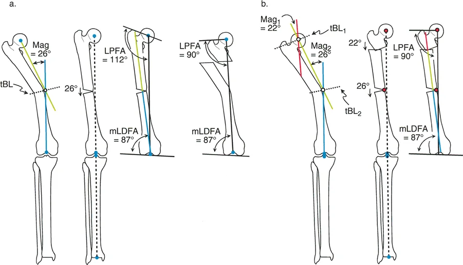
Identifying Proximal and Distal CORAs
To resolve this mathematically and plan a multi-level osteotomy, a third line known as the mid-diaphyseal line must be drawn. This line represents the normal, un-deformed segment of bone situated between the multiple apices of deformity.
- Draw the Proximal Mechanical Axis based on the normal proximal joint orientation angle.
- Draw the Distal Mechanical Axis based on the normal distal joint orientation angle.
- Identify the relatively straight, un-deformed segment of the diaphysis between the curves.
- Draw a line straight through the center of this intervening diaphyseal segment.
- The intersection of the Proximal Mechanical Axis with the mid-diaphyseal line creates the Proximal CORA.
- The intersection of the Distal Mechanical Axis with the mid-diaphyseal line creates the Distal CORA.
By isolating the normal intervening segment, the surgeon has effectively broken down one complex multiapical deformity into two distinct, manageable uniapical deformities, each with its own CORA and magnitude of angulation.
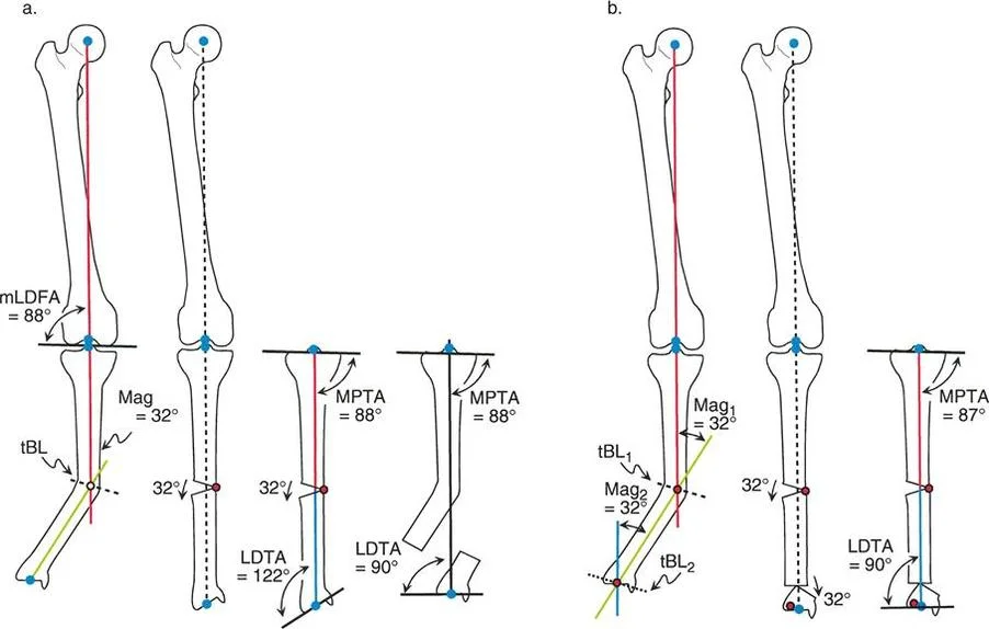
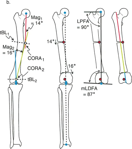
Step by Step Tibial Multiapical Deformity Analysis
Consider a complex deformity of the tibia involving both the proximal metaphysis and the distal diaphysis. To analyze this systematically:
- Proximal Axis: First, draw the proximal tibial axis based on the normal Medial Proximal Tibial Angle of 87 degrees.
- Distal Axis: Next, for the tibial Distal Mechanical Axis, draw a line from the center of the ankle joint extending proximally at 89 degrees, representing the normal Lateral Distal Tibial Angle.
- Observation: In a multiapical scenario, these proximal and distal lines will not intersect neatly within the tibial diaphysis. They may intersect outside the soft tissue envelope entirely.
- Mid-Diaphyseal Line: Identify the segment of the tibial shaft that appears straight. Draw the anatomic axis of this specific segment.
- Calculate Proximal Deformity: Measure the angle where the Proximal Mechanical Axis intersects the mid-diaphyseal line. This is the magnitude of the proximal deformity requiring a proximal osteotomy.
- Calculate Distal Deformity: Measure the angle where the Distal Mechanical Axis intersects the mid-diaphyseal line. This is the magnitude of the distal deformity requiring a distal osteotomy.
Advanced Preoperative Planning for Frontal Plane Osteotomies
Successful deformity correction occurs in the preoperative planning room, not in the operating theater. Dr. Paley established a rigorous, algorithm-based approach to analyzing full-length standing radiographs. This algorithm ensures that no component of the deformity is missed, including subtle joint subluxations or compensatory curves in adjacent bones.
The Malalignment Test
The Malalignment Test is the first step in the algorithm, designed to determine if a mechanical axis deviation exists and to quantify its severity.
- Step One: Obtain a high-quality, full-length, standing anteroposterior radiograph of both lower extremities with the patellae oriented strictly forward.
- Step Two: Draw the mechanical axis of the entire limb from the center of the femoral head to the center of the ankle plafond.
- Step Three: Measure the Mechanical Axis Deviation. If the line passes more than 8 millimeters medial to the center of the knee, a varus malalignment exists. If it passes lateral to the center of the knee, a valgus malalignment exists.
- Step Four: Evaluate the Joint Line Convergence Angle. If the JLCA is greater than 2 degrees, the malalignment is partially or entirely due to intra-articular factors, such as lateral compartment cartilage loss or medial collateral ligament laxity.
The Malorientation Test
If the Malalignment Test is positive (indicating an abnormal MAD), the surgeon must proceed to the Malorientation Test. This test identifies exactly which bone (femur, tibia, or both) is responsible for the deviation.
- Step One: Measure the mechanical Lateral Distal Femoral Angle. If the mLDFA is outside the normal range of 85 to 90 degrees, a femoral deformity is present.
- Step Two: Measure the Medial Proximal Tibial Angle. If the MPTA is outside the normal range of 85 to 90 degrees, a tibial deformity is present.
- Step Three: Measure the Lateral Distal Tibial Angle and the Lateral Proximal Femoral Angle to rule out compensatory deformities at the hip and ankle joints.
Key Takeaway: It is entirely possible to have a femoral deformity that cancels out a tibial deformity. For example, a valgus femur (mLDFA of 80 degrees) combined with a varus tibia (MPTA of 80 degrees) might result in a perfectly normal overall Mechanical Axis Deviation. However, the knee joint line will be severely oblique, leading to sheer forces and early osteoarthritis. The Malorientation Test uncovers these hidden, compensatory deformities.
Surgical Execution and Fixation Strategies
Once the CORA is identified and the osteotomy rules are applied, the surgeon must choose the appropriate method of fixation. The choice of hardware dictates how the osteotomy is performed and how the Angulation Correction Axis is controlled intraoperatively.
Choosing Between Internal and External Fixation
The decision between internal plates, intramedullary nails, and circular external fixators depends on the location of the CORA, the quality of the soft tissue envelope, and the presence of multi-planar deformities.
- Plating Systems: Opening or closing wedge osteotomies stabilized with locked plating systems (such as the TomoFix system) are ideal for uniapical deformities near the joint lines, such as the proximal tibia or distal femur. Plates provide rigid internal fixation but require precise, single-stage acute correction in the operating room.
- Intramedullary Nailing: Correcting deformities with intramedullary nails is mechanically advantageous due to load-sharing properties. However, the nail itself dictates the anatomic axis of the bone. To prevent the nail from following the path of the deformity, surgeons must utilize blocking screws (Poller screws). Placed strategically on the concavity of the deformity, Poller screws artificially narrow the medullary canal, forcing the nail to align the bone segments correctly.
- Circular External Fixation: For multiapical deformities, poor soft tissue envelopes, or cases requiring simultaneous limb lengthening, circular frames like the Ilizarov apparatus or the Taylor Spatial Frame are unmatched. The hinges of the frame can be placed exactly at the CORA, perfectly replicating Paley Rule One or Rule Two. Furthermore, hexapod frames allow for gradual, computer-assisted correction of six-axis deformities postoperatively, highly reducing the risk of acute neurovascular stretch injuries.
Managing the Soft Tissue Envelope
Bone correction cannot be viewed in isolation from the surrounding soft tissues. The neurovascular structures, muscles, and fascia dictate the limits of acute correction.
- The Peroneal Nerve: Acute correction of a severe valgus knee deformity (e.g., a distal femoral varus-producing osteotomy) places massive stretch on the common peroneal nerve. Surgeons must have a low threshold for performing a prophylactic common peroneal nerve decompression at the fibular neck to prevent postoperative foot drop.
- Fasciotomy: Acute angular corrections, particularly those involving translation (Paley Rule Two), significantly alter the volume of the fascial compartments. Prophylactic anterior and lateral compartment fasciotomies of the lower leg should be considered to prevent acute compartment syndrome.
Pitfalls and Complications in Deformity Correction
Even with meticulous preoperative planning, frontal plane realignment is fraught with potential intraoperative and postoperative complications. Recognizing these pitfalls early is essential for the orthopedic surgeon.
Avoiding Iatrogenic Translation
The most common error in deformity correction is failing to respect the Angulation Correction Axis, leading to an unintended Paley Rule Three scenario. If an opening wedge osteotomy is hinged on the wrong cortex, or if a closing wedge osteotomy removes an asymmetric wedge of bone not centered on the CORA, the distal segment will translate. This translation shifts the mechanical axis, potentially leaving the patient with residual Mechanical Axis Deviation despite the angular correction.
- Surgical Pearl: Always place a temporary hinge pin (such as a 2.0mm Kirschner wire) exactly at the planned Angulation Correction Axis before completing your bone cut. This physical barrier ensures the bone rotates purely around the intended axis without sliding or translating.
Recognizing Sagittal and Axial Plane Contributions
While this guide focuses heavily on frontal plane realignment, bone deformities are rarely isolated to a single plane. A varus tibia is frequently accompanied by a procurvatum (sagittal plane) deformity and internal tibial torsion (axial plane).
Failing to recognize a multi-planar deformity leads to the "projectional artifact" pitfall. If a bone is externally rotated, a pure sagittal plane bow will appear as a frontal plane deformity on an AP radiograph. Surgeons must obtain orthogonal radiographs and often utilize computed tomography (CT) scanograms to build a three-dimensional model of the deformity. When correcting multi-planar deformities acutely with internal fixation, the osteotomy plane must be mathematically calculated to address all planes simultaneously, often requiring an oblique, single-cut osteotomy.
Conclusion and Key Takeaways for Frontal Plane Realignment
Mastering frontal plane realignment osteotomy requires a deep, uncompromising adherence to the geometric principles established by Dr. Dror Paley. Transitioning from visual estimation to mathematical precision is the hallmark of an advanced reconstructive orthopedic surgeon.
Key Takeaways for the Orthopedic Surgeon:
* Trust the Axes: Never rely on the clinical appearance of the limb. Always draw the mechanical and anatomic axes, calculate the Mechanical Axis Deviation, and measure the joint orientation angles.
* Find the CORA: The Center of Rotation of Angulation dictates the entire surgical plan. Identifying the intersection of the Proximal and Distal Mechanical Axes is non-negotiable.
* Respect the Rules: Apply Paley Three Rules of Osteotomy to predict the mechanical outcome of your bone cuts. Use Rule One for pure angulation, Rule Two for planned translation, and avoid Rule Three unless correcting a pre-existing translational offset.
* Analyze Multiapical Deformities Systematically: Use the mid-diaphyseal line to break complex, multi-curve deformities down into manageable, uniapical components.
* Account for the Joint Line: Always measure the Joint Line Convergence Angle. A bony osteotomy will not fix a ligamentous deformity.
By rigorously applying these concepts, surgeons can execute complex deformity corrections with confidence, restoring optimal biomechanics, preserving joint longevity, and profoundly improving patient quality of life.
!!! info "Academic Resource & Medical Review"
This academic resource was prepared and medically reviewed by Prof. Dr. Mohammed Hutaif, Consultant Orthopedic & Spine Surgeon. It is formulated specifically for medical students, orthopedic residents, and surgeons preparing for high-stakes board examinations (AAOS, FRCS Tr & Orth, Arab Board).
!!! warning "Disclaimer"
The surgical techniques, classifications, and clinical guidelines presented herein are for educational and academic review purposes only. They are not intended to replace institutional protocols or independent clinical judgment.
You Might Also Like