Mastering Lower Limb Alignment: Paley's Principles for Orthopedic Deformity Correction
Key Takeaway
Paley's Principles provide a rigorous, geometric framework for orthopedic surgeons to analyze lower limb alignment and joint orientation. This involves identifying mechanical and anatomic axes, calculating joint angles (e.g., mLDFA, MPTA), and assessing mechanical axis deviation to precisely plan corrective osteotomies and arthroplasties for optimal biomechanical outcomes.
Introduction to Lower Limb Alignment and Joint Orientation
In the realm of orthopedic surgery, the mastery of lower limb alignment and joint orientation is what separates a good surgeon from a master reconstructive specialist. The foundation of modern deformity correction, heavily popularized and systematized by Dr. Dror Paley, relies on a rigorous, mathematical, and geometric understanding of how bones and joints relate to one another in three-dimensional space.
When a surgeon evaluates a limb for deformity, osteoarthritis, or plans for a complex osteotomy or arthroplasty, they cannot rely on subjective visual estimation. They must utilize reproducible, universally accepted joint orientation lines. These lines serve as the fundamental scaffolding upon which all deformity analysis is built, including the calculation of Mechanical Axis Deviation and the Center of Rotation of Angulation.
This comprehensive masterclass transforms the foundational concepts of normal lower limb alignment into a high-yield, deeply clinical guide for surgeons-in-training. We will dissect the exact methodology for drawing joint orientation lines across the ankle, knee, and hip in both the frontal and sagittal planes, and explore the profound biomechanical implications of these measurements. By mastering these principles, orthopedic surgeons can execute precise, predictable, and biomechanically sound reconstructive procedures.
The Foundation of Mechanical and Anatomic Axes
Before one can understand joint orientation, one must first master the axes of the lower extremity. A joint orientation line does not exist in a vacuum. Its primary clinical utility is derived from the angle it forms when it intersects with a bone's mechanical or anatomic axis. Accurate identification of these axes on full-length, weight-bearing radiographs is the absolute first step in deformity planning.
Mechanical Axis of the Lower Extremity
The mechanical axis of a bone is defined by a straight line connecting the center points of its proximal and distal joints.
- Mechanical Axis of the Lower Limb A line drawn from the center of the femoral head to the center of the ankle mortise. In a normal, well-aligned limb, this line passes slightly medial to the center of the knee joint, typically 8mm plus or minus 7mm medial to the center.
- Mechanical Axis of the Femur A line drawn from the center of the femoral head to the center of the knee joint at the intercondylar notch.
- Mechanical Axis of the Tibia A line drawn from the center of the proximal tibia to the center of the tibial plafond at the ankle.
Anatomic Axis of the Lower Extremity
The anatomic axis is the mid-diaphyseal line of the bone, representing the actual physical shaft of the osseous structure.
- Anatomic Axis of the Femur Drawn through the center of the femoral diaphysis. Because of the natural anterior bow and the offset of the femoral head, the anatomic axis of the femur sits at an angle of roughly 5 to 7 degrees relative to the mechanical axis of the femur. This is clinically vital during intramedullary nailing and total knee arthroplasty planning.
- Anatomic Axis of the Tibia Drawn through the center of the tibial diaphysis. In the tibia, the anatomic and mechanical axes are essentially parallel and often superimposed, making tibial deformity analysis slightly more straightforward than femoral analysis.
Mechanical Axis Deviation and The Malalignment Test
When the mechanical axis of the lower limb fails to pass through the center of the knee joint and falls outside the normal physiologic parameters, the limb is said to have Mechanical Axis Deviation. Identifying Mechanical Axis Deviation is the trigger that prompts a surgeon to evaluate the individual joint orientation lines to locate the exact source of the deformity.
The Malalignment Test is performed by drawing the mechanical axis of the entire lower limb on a standing long-leg radiograph.
- Medial Deviation Indicates a varus deformity. The weight-bearing line passes through the medial compartment of the knee, exponentially increasing contact stresses and leading to medial compartment osteoarthritis.
- Lateral Deviation Indicates a valgus deformity. The weight-bearing line passes through the lateral compartment, leading to lateral cartilage wear and medial collateral ligament stretch.
Clinical Pearls for Mechanical Axis Deviation
* Always ensure the radiograph is taken with the patella facing directly forward. Rotational malpositioning will artificially alter the appearance of the mechanical axis.
* Mechanical Axis Deviation is measured in millimeters from the center of the knee joint.
* A normal knee has a slight physiologic varus moment, which is why the normal mechanical axis falls just medial to the exact center of the tibial spines.
Systematic Nomenclature of Joint Orientation Lines
A joint orientation line is a geometric representation of the articular surface of a joint in a specific plane or radiographic projection. By drawing these lines and measuring the angles they form with the mechanical and anatomic axes, surgeons can quantify normal anatomy and identify pathologic deviations.
The nomenclature for these angles is highly systematic in Paley's principles. They are named using a combination of letters to ensure universal communication among reconstructive surgeons.
- m or a Mechanical or Anatomic axis.
- M or L or A or P Medial, Lateral, Anterior, or Posterior, indicating which side of the angle is being measured.
- P or D Proximal or Distal.
- F or T Femur or Tibia.
- A Angle.
For example, mLDFA stands for the mechanical Lateral Distal Femoral Angle.
| Angle Abbreviation | Full Name | Normal Range | Average Value |
|---|---|---|---|
| mLDFA | Mechanical Lateral Distal Femoral Angle | 85° - 90° | 87° |
| aLDFA | Anatomic Lateral Distal Femoral Angle | 79° - 83° | 81° |
| MPTA | Medial Proximal Tibial Angle | 85° - 90° | 87° |
| LDTA | Lateral Distal Tibial Angle | 86° - 92° | 89° |
| ADTA | Anterior Distal Tibial Angle | 78° - 82° | 80° |
| PPTA | Posterior Proximal Tibial Angle | 77° - 84° | 81° |
| JLCA | Joint Line Convergence Angle | 0° - 2° | 1° |
Ankle Joint Biomechanics and Orientation
The ankle or tibiotalar joint is a complex hinge joint that must absorb tremendous ground reaction forces during the gait cycle. Precise alignment is critical to prevent asymmetric loading, which rapidly leads to post-traumatic or primary osteoarthritis.
Frontal Plane Ankle Orientation
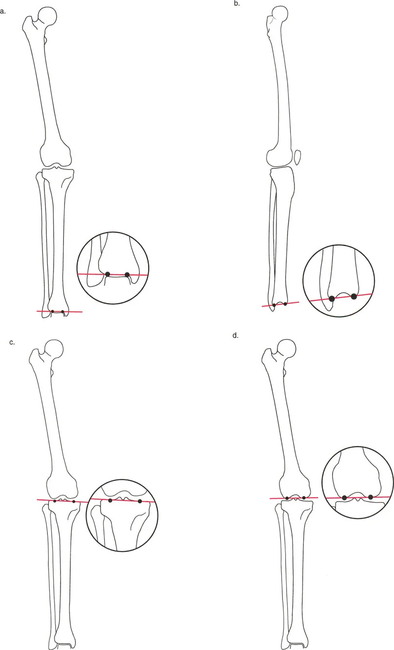
At the ankle, the joint orientation line in the frontal or coronal plane is drawn across the flat subchondral line of the tibial plafond. This can be drawn on either the distal tibial subchondral line itself or, alternatively, along the subchondral line of the dome of the talus.
When this joint orientation line intersects the mechanical axis of the tibia, it forms the Lateral Distal Tibial Angle.
- Normal Lateral Distal Tibial Angle 86° to 92°, with an average of 89°.
- Clinical Implication A Lateral Distal Tibial Angle less than 86° indicates distal tibial varus, which shifts contact pressures medially. An angle greater than 92° indicates distal tibial valgus, shifting pressures laterally. Correcting this angle is a primary goal in supramalleolar osteotomies.
Sagittal Plane Ankle Orientation
In the sagittal plane, the ankle joint orientation line is drawn from the distal tip of the posterior lip of the tibia to the distal tip of the anterior lip of the tibia.
When this line intersects the anatomic or mechanical axis of the tibia in the sagittal plane, it forms the Anterior Distal Tibial Angle.
- Normal Anterior Distal Tibial Angle 78° to 82°, with an average of 80°.
- Clinical Implication The Anterior Distal Tibial Angle dictates the sagittal tilt of the ankle plafond. If the angle is increased, for example greater than 85°, the joint is in procurvatum, leading to anterior impingement and altered gait mechanics. Conversely, a decreased angle less than 75° indicates recurvatum, shifting the load posteriorly and often resulting in Achilles tendon contractures and posterior cartilage wear.
Knee Joint Orientation and Coronal Plane Angles
The knee joint is the largest and most complex joint in the human body, serving as the central pivot point for the lower extremity mechanical axis. Deformities around the knee are the most common indications for corrective osteotomies.
Distal Femoral Angles
The distal femoral joint orientation line is drawn tangentially across the most distal points of the medial and lateral femoral condyles.
- Mechanical Lateral Distal Femoral Angle This is the angle formed by the mechanical axis of the femur and the distal femoral joint orientation line. The normal average is 87°. An increased angle indicates femoral varus, while a decreased angle indicates femoral valgus.
- Anatomic Lateral Distal Femoral Angle This is the angle formed by the anatomic axis of the femur and the joint line. The normal average is 81°. This measurement is heavily utilized in total knee arthroplasty when setting the distal femoral cutting block referencing the intramedullary canal.
Proximal Tibial Angles
The proximal tibial joint orientation line is drawn across the subchondral bone of the medial and lateral tibial plateaus, ignoring the intercondylar eminence.
- Medial Proximal Tibial Angle Formed by the intersection of the mechanical axis of the tibia and the proximal tibial joint line. The normal average is 87°.
- Clinical Implication A decreased Medial Proximal Tibial Angle is the hallmark of tibia vara, commonly seen in Blount's disease or medial compartment osteoarthritis. High Tibial Osteotomy aims to correct this angle to restore normal joint loading.
Joint Line Convergence Angle
The Joint Line Convergence Angle is measured between the distal femoral joint orientation line and the proximal tibial joint orientation line.
- Normal Joint Line Convergence Angle 0° to 2°. The lines should be nearly parallel.
- Clinical Implication An increased Joint Line Convergence Angle indicates intra-articular deformity, which may be due to asymmetric cartilage loss, such as medial joint space narrowing in osteoarthritis, or ligamentous laxity, such as lateral collateral ligament stretch in a chronic varus knee. When planning an extra-articular osteotomy, the surgeon must account for the Joint Line Convergence Angle, or they risk under-correcting or over-correcting the limb.
Knee Joint Orientation in the Sagittal Plane
Sagittal plane deformities of the knee profoundly affect the extensor mechanism and the patient's ability to achieve full extension or flexion.
Posterior Proximal Tibial Angle
The proximal tibial joint orientation line in the sagittal plane is drawn from the anterior to the posterior aspect of the tibial plateau. When intersected with the tibial anatomic axis, it forms the Posterior Proximal Tibial Angle.
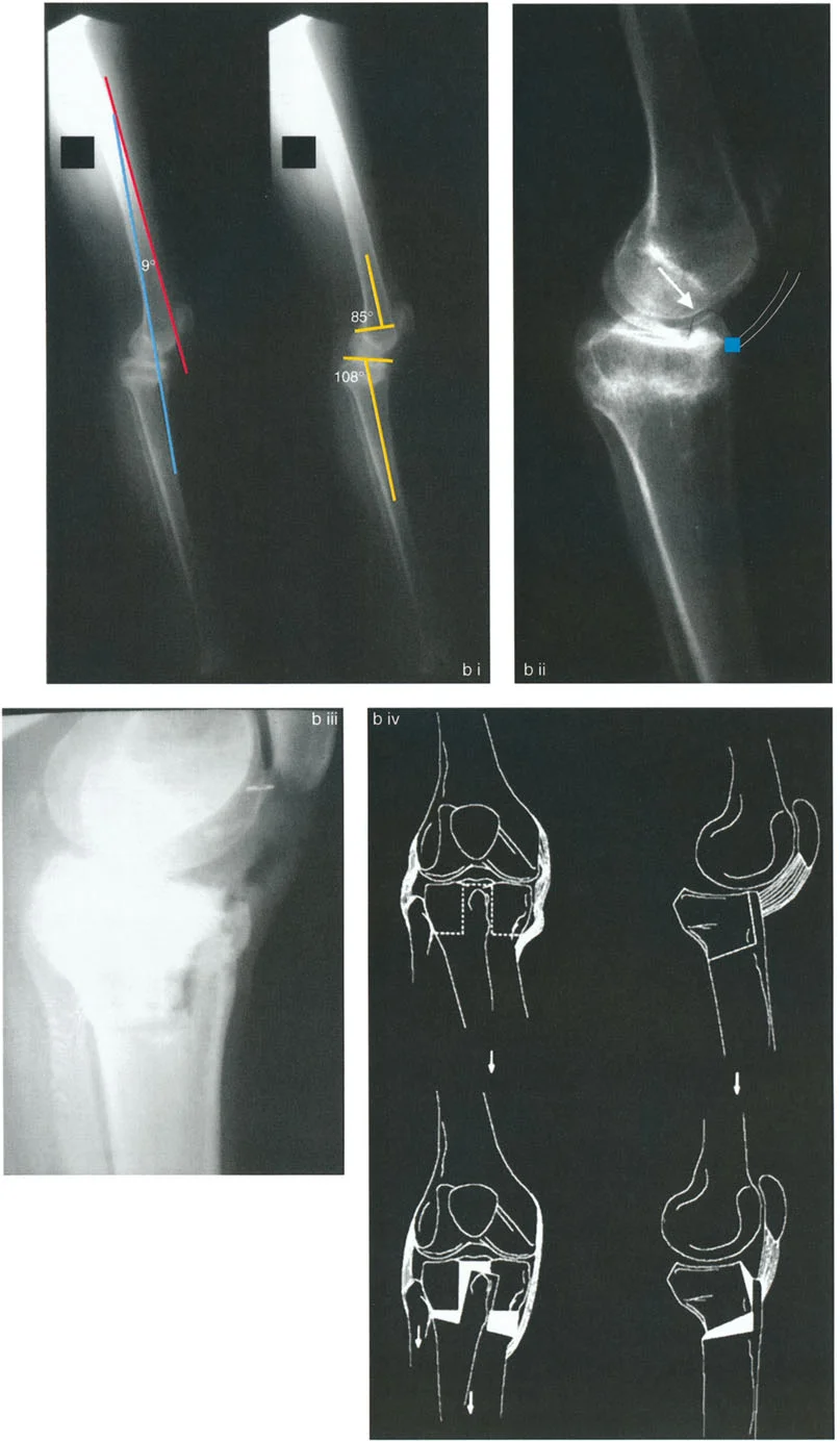
- Normal Posterior Proximal Tibial Angle 77° to 84°, with an average of 81°. This represents the normal posterior slope of the tibial plateau, which is roughly 9°.
- Clinical Implication Maintaining the normal posterior slope is critical during a High Tibial Osteotomy. Inadvertently increasing the slope will alter knee kinematics, increase strain on the anterior cruciate ligament, and limit knee extension. Decreasing the slope places excessive strain on the posterior cruciate ligament.
Distal Femoral Sagittal Angles
In the sagittal plane, the distal femoral joint line is drawn from the anterior to the posterior extent of the femoral condyles. The angle formed with the anatomic axis of the femur dictates the sagittal bowing of the distal femur. Abnormalities here manifest as femoral extension or flexion deformities, directly impacting the patellofemoral joint mechanics.
Hip Joint Orientation and Proximal Femoral Geometry
The proximal femur is defined by a complex three-dimensional geometry that dictates hip biomechanics, abductor lever arm length, and leg length equality.
Proximal Femoral Angles
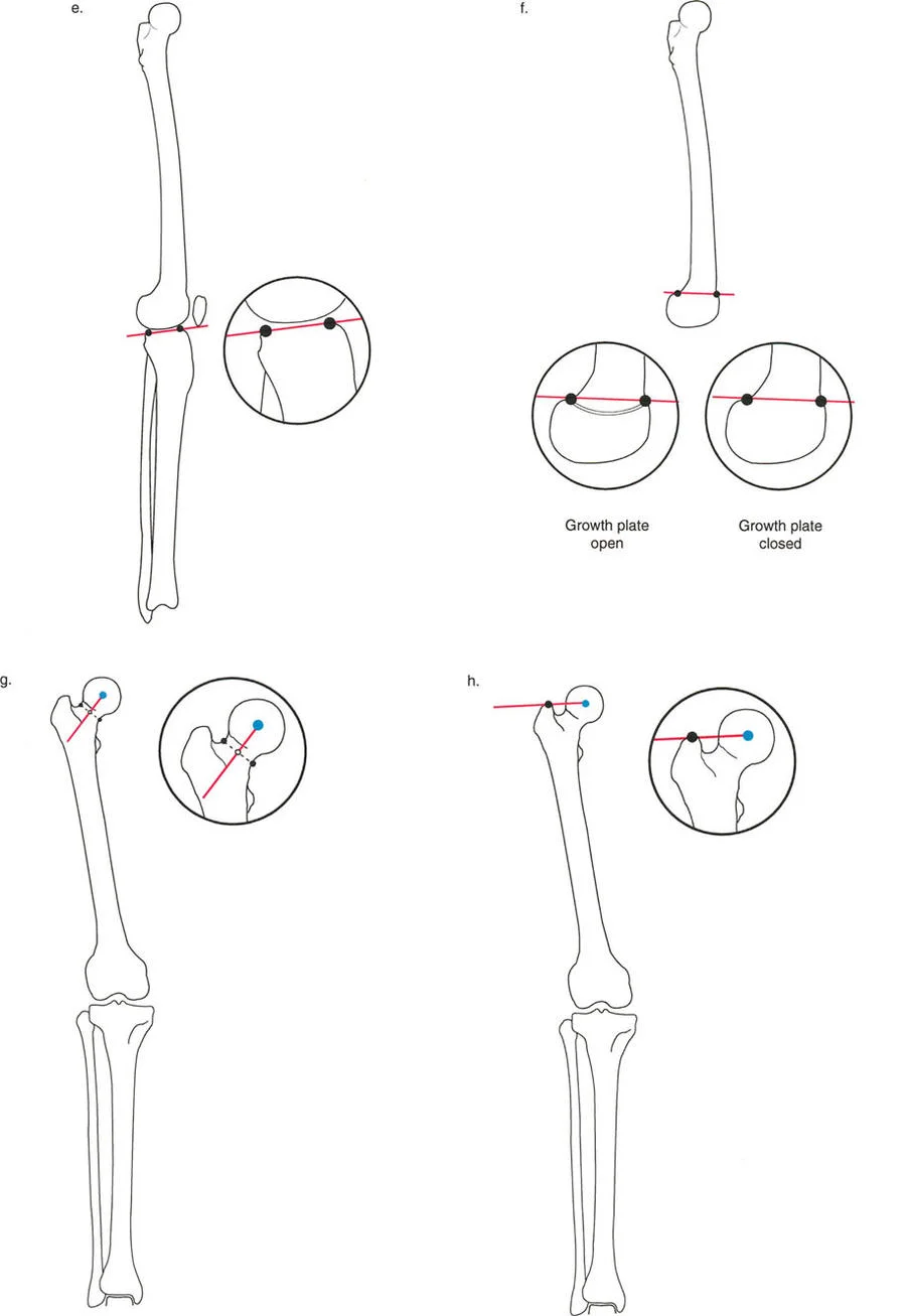
The proximal femoral joint orientation line is drawn from the tip of the greater trochanter to the center of the femoral head.
- Mechanical Lateral Proximal Femoral Angle Formed by the intersection of the mechanical axis of the femur and the proximal joint orientation line. The normal average is 90°.
- Clinical Implication Deviations in this angle indicate coxa vara or coxa valga relative to the mechanical axis. A decreased angle represents coxa vara, which shortens the limb and weakens the abductor moment, leading to a Trendelenburg gait.
Neck Shaft Angle
While not a traditional joint orientation line, the Neck Shaft Angle is a critical anatomic measurement. It is the angle formed between the anatomic axis of the femoral shaft and the anatomic axis of the femoral neck.
- Normal Neck Shaft Angle 125° to 135°, with an average of 130°.
- Clinical Implication The Neck Shaft Angle is vital for planning proximal femoral osteotomies. Altering this angle changes the articulotrochanteric distance, which directly impacts the tension of the gluteus medius and minimus muscles.
Center of Rotation of Angulation CORA Principles
Identifying the mechanical axis deviation and abnormal joint orientation angles only tells the surgeon that a deformity exists and which bone is affected. To correct the deformity, the surgeon must determine exactly where the deformity is located within the bone. This is achieved by finding the Center of Rotation of Angulation.
The Center of Rotation of Angulation is the intersection point of the proximal mechanical axis line and the distal mechanical axis line of a deformed bone. Alternatively, anatomic axes can be used to find the anatomic Center of Rotation of Angulation.
Key Concepts of CORA Mapping
* Single CORA If a bone has a single uniapical deformity, the proximal and distal axes will intersect at a single point. This point represents the apex of the deformity.
* Multiple CORAs In complex, multi-apical deformities, the proximal and distal axes will not intersect at the actual site of the bone deformity. Instead, a mid-diaphyseal line must be drawn, creating multiple intersection points. This indicates that multiple osteotomies may be required to fully restore normal alignment without causing secondary translation.
* Magnitude and Direction The angle formed at the intersection of the proximal and distal axes is the magnitude of the deformity. The bisector of this angle provides the optimal plane for correction.
Paley Osteotomy Rules for Deformity Correction
Dr. Dror Paley established three fundamental geometric rules for osteotomy placement relative to the Center of Rotation of Angulation. Mastering these rules allows the surgeon to predict exactly how the bone segments will behave during correction.
Osteotomy Rule One
When the osteotomy and the axis of correction hinge are both located at the CORA.
* Biomechanical Result The bone will undergo pure angulation. The mechanical axis of the proximal segment will perfectly align with the mechanical axis of the distal segment without any translation.
* Clinical Application This is the ideal scenario for a simple closing wedge or opening wedge osteotomy at the apex of the deformity. It perfectly restores the bone's mechanical axis.
Osteotomy Rule Two
When the osteotomy is located away from the CORA, but the axis of correction hinge remains at the CORA.
* Biomechanical Result The bone segments will undergo both angulation and translation. By keeping the hinge at the CORA, the proximal and distal mechanical axes will still perfectly realign, but the bone ends at the osteotomy site will be displaced relative to one another.
* Clinical Application This is highly useful when the CORA is located very close to a joint line, where there is insufficient bone stock for fixation. The surgeon can perform the cut in the diaphysis while hinging the correction around the joint line CORA. The resulting translation is an expected and necessary geometric consequence to restore the straight mechanical axis.
Osteotomy Rule Three
When the osteotomy and the axis of correction hinge are both located away from the CORA.
* Biomechanical Result The bone will undergo angulation, but the proximal and distal mechanical axes will not align. A secondary translation deformity is created.
* Clinical Application This rule represents a geometric failure and is generally avoided. If a surgeon simply cuts a bone and hinges it open away from the true apex of the deformity, they will induce a zigzag deformity in the mechanical axis, shifting the weight-bearing line pathologically.
Step by Step Preoperative Planning for Deformity Correction
To synthesize Paley's principles into a practical surgical workflow, the orthopedic surgeon must follow a rigorous, step-by-step preoperative planning protocol. Skipping steps leads to geometric errors and poor clinical outcomes.
- Obtain Proper Radiographs Acquire weight-bearing, full-length lower extremity radiographs. The patella must be pointing strictly forward to control for rotation. Obtain dedicated orthogonal views of the affected bone.
- Perform the Malalignment Test Draw the mechanical axis of the entire lower limb from the femoral head to the ankle mortise. Measure the Mechanical Axis Deviation in millimeters from the center of the knee.
- Perform the Malorientation Test Draw the joint orientation lines for the hip, knee, and ankle. Measure the specific angles including the mechanical Lateral Distal Femoral Angle and the Medial Proximal Tibial Angle. Compare these to normal population averages or the contralateral normal limb.
- Identify the Deformed Bone Based on the abnormal joint orientation angles, determine whether the deformity lies in the femur, the tibia, or both. Evaluate the Joint Line Convergence Angle to rule out intra-articular soft tissue contributions.
- Determine the CORA Draw the proximal and distal mechanical axes of the deformed bone. Mark their intersection point to find the Center of Rotation of Angulation. Measure the magnitude of the angular deformity.
- Apply Osteotomy Rules Decide on the level of the osteotomy. If cutting at the CORA, plan a simple angular correction. If cutting away from the CORA due to bone quality or soft tissue envelope constraints, calculate the required translation using Rule Two.
- Assess Leg Length Discrepancy Measure the length of the femur and tibia. If the angular correction will result in significant shortening, plan for a simultaneous distraction osteogenesis procedure or a carefully calculated opening wedge osteotomy.
Conclusion
The transition from visual estimation to precise geometric planning is the hallmark of advanced reconstructive orthopedic surgery. Dr. Dror Paley's principles of lower limb alignment provide a universal language and a mathematical framework for tackling even the most complex deformities.
By systematically applying the concepts of Mechanical Axis Deviation, Joint Orientation Angles, and the Center of Rotation of Angulation, surgeons can demystify lower extremity pathology. Adherence to the three Osteotomy Rules ensures that surgical interventions are not merely reactive, but are highly calculated biomechanical restorations that preserve joint health, optimize gait kinematics, and profoundly improve patient outcomes.
!!! info "Academic Resource & Medical Review"
This academic resource was prepared and medically reviewed by Prof. Dr. Mohammed Hutaif, Consultant Orthopedic & Spine Surgeon. It is formulated specifically for medical students, orthopedic residents, and surgeons preparing for high-stakes board examinations (AAOS, FRCS Tr & Orth, Arab Board).
!!! warning "Disclaimer"
The surgical techniques, classifications, and clinical guidelines presented herein are for educational and academic review purposes only. They are not intended to replace institutional protocols or independent clinical judgment.
You Might Also Like